数据分析04--Pandas文件读取和绘图
python-databasePandas文件读取和绘图,包括文件读取、分箱操作、时间序列、基础绘图等
写在前面:本笔记来自b站课程千锋教育python数据分析教程200集
资料下载 提取码:wusa
文件读取
csv/table
df.to_csv(存放路径, sep=',', header=True, index=True)
-
sep:分隔符,一般csv的都为逗号 -
header:是否保留列索引 -
index:是否保留行索引
    A   B   C
1  A1  B1  C1
2  A2  B2  C2
3  A3  B3  C3
4  A4  B4  C4
5  A5  B5  C5
df.to_csv('data.csv')

pd.read_csv(数据路径, sep=',', header=0, index_col=None)
-
sep:分隔符,一般csv的都为逗号 -
header:指定哪行作为列索引,默认为第一行 -
index_col:指定哪列作为行索引,默认不读取行索引,都作为元素读取 -
header和index_col都可取整数值/字符串,表示第几行/列或者行/列名;也可取None,表示不读取行/列索引;也可以是一个整数型列表,表示将指定行/列都作为行/列索引(多层索引)
读取上面的数据:
print(pd.read_csv('data.csv', index_col=0))
    A   B   C
1  A1  B1  C1
2  A2  B2  C2
3  A3  B3  C3
4  A4  B4  C4
5  A5  B5  C5
read_table用法同read_csv,只是分隔符默认为制表符\t
没有to_table
excel
df.to_excel(存放路径, sheet_name="Sheet1", header=True, index=True)
-
sheet_name:工作表名称 -
header:是否保留列索引 -
index:是否保留行索引
注:该函数需要安装openpyxl包
df.to_excel('data.xlsx')

pd.read_excel(数据路径, sheet_name=0, header=0, index_col=None, names=None)
-
sheet_name:读取哪个工作表。可以是数字,表示读取第几个表;也可以是工作表名称 -
header和index_col参数同csv/table -
names:设置列名
# pd.read_excel('data.xlsx', index_col=0)
    A   B   C
1  A1  B1  C1
2  A2  B2  C2
3  A3  B3  C3
4  A4  B4  C4
5  A5  B5  C5
# pd.read_excel('data.xlsx', header=0, names=list("abcd"), index_col=0)
    b   c   d
a
1  A1  B1  C1
2  A2  B2  C2
3  A3  B3  C3
4  A4  B4  C4
5  A5  B5  C5
sql
需要SQLAlchemy和pymysql包
create_engine('数据库类型+驱动://用户名:密码@数据库地址:端口号/数据库名')
以mysql数据库为例:root用户、默认端口号、本地数据库
from sqlalchemy import create_engine
conn = create_engine("mysql+pymysql://root:123456@localhost:3306/test")
df.to_sql(name,con,index=True,if_exists='fail')
-
name:数据库中表名 -
con:数据库连接对象,即上面获取的conn -
index:是否保存行索引 -
if_exists:如果表已经存在时的处理方法,如果设为append则为追加写入
df.to_sql(
    name='df',  # 保存到df表中
    con=conn,  # 设置连接对象
    index=False,  # 不保存行索引
    if_exists='append'  # 追加写入
)

pd.read_sql(sql,con,index_col=None)
-
sql:一般是sql查询语句,将其返回结果进行保存 -
con:数据库连接对象,即上面获取的conn -
index_col=None指定哪列作为行索引,默认不设置行索引(行索引为0-n)
print(pd.read_sql(
    sql="select * from df",  # 读取df表的全部数据
    con=conn,  # 设置连接对象
))
    A   B   C
0  A1  B1  C1
1  A2  B2  C2
2  A3  B3  C3
3  A4  B4  C4
4  A5  B5  C5
print(pd.read_sql(
    sql="select * from df",
    con=conn,
    index_col="A"  # 指定A列作行索引
))
     B   C
A
A1  B1  C1
A2  B2  C2
A3  B3  C3
A4  B4  C4
A5  B5  C5
分箱操作
即将连续型数据离散化,分为等距和等频分箱
可以理解成将数据按指定范围分组
等距分箱
pd.cut(series, bins=n/list, right=True, labels=list)表示将series平均分为n组
-
bins也可以是一个列表[n1,n2,n3,...],表示分成(n1,n2](n2,n3](n3,...]的多组 -
right设置分组区间开闭,默认是左开右闭,可以设置为False即左闭右开 -
labels设置分组区间名称,是一个字符串列表
    A   B   C
a  14  74  29
b  22  12  68
c  65  80  22
d  79  29  19
e  99  89  56
# print(pd.cut(df['A'], bins=4, right=False))
a      [14.0, 35.25)
b      [14.0, 35.25)
c      [56.5, 77.75)
d    [77.75, 99.085)
e    [77.75, 99.085)
Name: A, dtype: category
Categories (4, interval[float64]): [[14.0, 35.25) < [35.25, 56.5) < [56.5, 77.75) < [77.75, 99.085)]
最后一行Categories展示了各组的范围,上面的series展示了abcde对应的数据都在哪组
可以看到默认情况下每组的距离相等
# print(pd.cut(df['A'], bins=[0, 30, 60, 80, 100], labels=['0-30', '30-60', '60-80', '80-100']))
a      0-30
b      0-30
c     60-80
d     60-80
e    80-100
Name: A, dtype: category
Categories (4, object): ['0-30' < '30-60' < '60-80' < '80-100']
这里我们指定了分组的名称
等距分箱
pd.qcut(series, q=n, labels=list)表示将series平均分为n组
-
q设置将数据均分成n等份 -
right设置分组区间开闭,默认是左开右闭,可以设置为False即左闭右开 -
labels设置分组区间名称,是一个字符串列表
    A   B   C
a  73   1  68
b   8  83  77
c  14  86  90
d  29  95  60
e  54  12  92
# pd.qcut(df['A'], q=4)
a     (54.0, 73.0]
b    (7.999, 14.0]
c    (7.999, 14.0]
d     (14.0, 29.0]
e     (29.0, 54.0]
Name: A, dtype: category
Categories (4, interval[float64]): [(7.999, 14.0] < (14.0, 29.0] < (29.0, 54.0] < (54.0, 73.0]]
可以看到各组中分别有2、1、1、1个数据,因为是5个数据分成4组,无法完全均分,所以就让第一组多一个数据
等距和等频分箱的区别在于:
-
等距分箱只确保每组的距离相等(默认情况下),不管每组中是否有数据
-
等距分箱只确保每组中数据数量尽可能相等,不管每组的具体范围是多少
时间序列
时间戳
pd.Timestamp("Y-M-D hour:minute:second")创建指定时刻的时间戳,其中年份Y必须指定
print(pd.Timestamp("2000"))  # 2000-01-01 00:00:00
print(pd.Timestamp("2010-10-10"))  # 2010-10-10 00:00:00
print(pd.Timestamp("2022-12-23 20:30:45"))  # 2022-12-23 20:30:45
pd.Period("Y-M-D", freq='D')创建时期数据,参数freq指定创建的是年Y、月M、日D
print(pd.Period('2010', freq='D'))  # 2010-01-01
print(pd.Period("2010-10-10", freq='M'))  # 2010-10
print(pd.Period("2022-12-23", freq='Y'))  # 2022
批量生成时刻/时期数据:
时刻数据:pd.date_range('Y.M.D', periods=n, freq='D')从指定时间开始,连续取n天/月/年,得到一个DatetimeIndex对象。特点是最后必须具体到天
时期数据:pd.period_range('Y.M.D', periods=n, freq='D')从指定时间开始,连续取n天/月/年,得到一个PeriodIndex对象。特点是可以只具体到年/月/日
print(pd.date_range('2030.02.13', periods=4, freq='D'))
# DatetimeIndex(['2030-02-13', '2030-02-14', '2030-02-15', '2030-02-16'], dtype='datetime64[ns]', freq='D')
print(pd.date_range('2030.02.13', periods=4, freq='M'))
# DatetimeIndex(['2030-02-28', '2030-03-31', '2030-04-30', '2030-05-31'], dtype='datetime64[ns]', freq='M')
print(pd.date_range('2030.02.13', periods=4, freq='Y'))
# DatetimeIndex(['2030-12-31', '2031-12-31', '2032-12-31', '2033-12-31'], dtype='datetime64[ns]', freq='A-DEC')
print(pd.period_range('2030.02.13', periods=4, freq='Y'))
# PeriodIndex(['2030', '2031', '2032', '2033'], dtype='period[A-DEC]', freq='A-DEC')
可以看到时刻数据中按月取默认是最后一天,按年取默认是最后一月的最后一天
时间戳索引:上面创建的时间数据一般不会单独使用,而是作为数据的索引
index = pd.date_range('2010.01.02', periods=5)
print(pd.Series(np.random.randint(0, 10, size=5), index=index))
2010-01-02    6
2010-01-03    4
2010-01-04    6
2010-01-05    7
2010-01-06    0
Freq: D, dtype: int32
各种时间数据的转换
可以将不规则的时间字符串转换成时刻数据
pd.to_datetime(str)其中str也可以是一个字符串列表
print(pd.to_datetime('2030-03-14'))
# 2030-03-14 00:00:00
print(pd.to_datetime(['2030-03-14', '2030-3-14', '14/03/2030', '2030/3/14']))
# DatetimeIndex(['2030-03-14', '2030-03-14', '2030-03-14', '2030-03-14'], dtype='datetime64[ns]', freq=None)
时间戳也可以转换成时刻数据
pd.to_datetime(时间戳, unit) 其中unit参数指定时间戳的单位
print(pd.to_datetime([1899678987], unit='s'))
# DatetimeIndex(['2030-03-14 00:36:27'], dtype='datetime64[ns]', freq=None)
print(pd.to_datetime(1899678987000, unit='ms'))
# 2030-03-14 00:36:27
时间差
pd.DateOffset(years/months/days/hours/seconds/minutes)
dt = pd.Timestamp("2022-12-23 20:30:45")
print(dt + pd.DateOffset(years=8))  # 2030-12-23 20:30:45
print(dt + pd.DateOffset(months=-8))  # 2022-04-23 20:30:45
print(dt - pd.DateOffset(days=8))  # 2022-12-15 20:30:45
print(dt + pd.DateOffset(hours=8))  # 2022-12-24 04:30:45
print(dt + pd.DateOffset(seconds=8))  # 2022-12-23 20:30:53
print(dt + pd.DateOffset(minutes=8))  # 2022-12-23 20:38:45
表示在基础时间上加减
取值与切片
准备数据:
index = pd.date_range('2010.01.02', periods=100)
ts = pd.Series(range(len(index)), index=index)  # ts表示以DatetimeIndex对象为索引的series
print(ts)
2010-01-02     0
2010-01-03     1
2010-01-04     2
2010-01-05     3
2010-01-06     4
              ..
2010-04-07    95
2010-04-08    96
2010-04-09    97
2010-04-10    98
2010-04-11    99
Freq: D, Length: 100, dtype: int64
根据索引取值:ts[索引名]索引名可以不是具体的2010-04-11日期,也可以是月/年
print(ts["2010-01-03"])  # 1
print(ts["2010-1-3"])  # 1    可以省略月/日中的0
print(ts["2010-2"])  # 取整个2月的所有数据
2010-02-01    30
2010-02-02    31
2010-02-03    32
              ..
2010-02-26    55
2010-02-27    56
2010-02-28    57
Freq: D, dtype: int64
切片:ts[索引名1:索引名2]取[索引名1,索引名2]中的所有数据
# ts["2010-1-3":"2010-1-7"]
2010-01-03    1
2010-01-04    2
2010-01-05    3
2010-01-06    4
2010-01-07    5
Freq: D, dtype: int64
# ts["2010-2":"2010-3"]
2010-02-01    30
2010-02-02    31
2010-02-03    32
              ..
2010-03-29    86
2010-03-30    87
2010-03-31    88
Freq: D, dtype: int64
时间戳作索引进行取值/切片:ts[时间戳]或ts[时间戳1:时间戳2]
print(ts[pd.Timestamp("2010-1-3")]) # 1
DatetimeIndex作索引进行切片:ts[DatetimeIndex]
# ts[pd.date_range('2010.02.03', periods=5, freq='D')]
2010-02-03    32
2010-02-04    33
2010-02-05    34
2010-02-06    35
2010-02-07    36
Freq: D, dtype: int64
常用属性
准备数据:
index = pd.date_range('2010.01.29', periods=5)
ts = pd.Series(range(len(index)), index=index)
print(ts)
2010-01-29    0
2010-01-30    1
2010-01-31    2
2010-02-01    3
2010-02-02    4
Freq: D, dtype: int64
-
ts.index获取该series的索引(DatetimeIndex对象)# ts.index DatetimeIndex(['2010-01-29', '2010-01-30', '2010-01-31', '2010-02-01', '2010-02-02'], dtype='datetime64[ns]', freq='D') -
ts.index.year该DatetimeIndex对象的日期都是哪年的print(ts.index.year) # Int64Index([2010, 2010, 2010, 2010, 2010], dtype='int64') -
ts.index.month是哪月的print(ts.index.month) # Int64Index([1, 1, 1, 2, 2], dtype='int64') -
ts.index.day是哪日的print(ts.index.day) # Int64Index([29, 30, 31, 1, 2], dtype='int64') -
ts.index.dayofweek是星期几的print(ts.index.dayofweek) # Int64Index([4, 5, 6, 0, 1], dtype='int64')
常用方法
移动
ts.shift(periods=1)将数据整体往后移一位,若给负数就是往前移
准备数据:
index = pd.date_range('2010.01.29', periods=5)
ts = pd.Series(range(len(index)), index=index)
print(ts)
2010-01-29    0
2010-01-30    1
2010-01-31    2
2010-02-01    3
2010-02-02    4
Freq: D, dtype: int64
# ts.shift()
2010-01-29    NaN
2010-01-30    0.0
2010-01-31    1.0
2010-02-01    2.0
2010-02-02    3.0
Freq: D, dtype: float64
# ts.shift(periods=-3)
2010-01-29    3.0
2010-01-30    4.0
2010-01-31    NaN
2010-02-01    NaN
2010-02-02    NaN
Freq: D, dtype: float64
频率转换
即对数据进行抽样
-
由多变少:
-
ts.asfreq(pd.tseries.offsets.Week())天->星期 -
ts.asfreq(pd.tseries.offsets.MonthEnd())天->月
-
-
有少变多:用
fill_value填充ts.asfreq(pd.tseries.offsets.Hour(), fill_value=0)天->小时
# ts.asfreq(pd.tseries.offsets.Week())
2010-01-29    0
Freq: W, dtype: int64
# ts.asfreq(pd.tseries.offsets.MonthEnd())
2010-01-31    2
Freq: M, dtype: int64
# ts.asfreq(pd.tseries.offsets.Hour(), fill_value=0)
2010-01-29 00:00:00    0
2010-01-29 01:00:00    0
2010-01-29 02:00:00    0
                      ..
2010-02-01 22:00:00    0
2010-02-01 23:00:00    0
2010-02-02 00:00:00    4
Freq: H, Length: 97, dtype: int64
重采样(最常用)
即对数据按一定间隔进行聚合
ts.resample('时间间隔').聚合函数()
-
时间间隔:
数量+S/T/H/D/W/M/Y表示几秒/分钟/小时/天/周/月/年,如果不写数量默认为1 -
聚合函数:
sum()、cumsum()等
数据:
index = pd.date_range('2010.01.29', periods=365)
ts = pd.Series(range(len(index)), index=index)
# ts.resample('2D').sum()
2010-01-29      1
2010-01-31      5
2010-02-02      9
             ...
2011-01-24    721
2011-01-26    725
2011-01-28    364
Freq: 2D, Length: 183, dtype: int64
# ts.resample('3M').sum().cumsum()
2010-01-31        3
2010-04-30     4186
2010-07-31    16836
2010-10-31    37950
2011-01-31    66430
Freq: 3M, dtype: int64
df的重采样:
df.resample('时间间隔', on='列名').聚合函数()
数据:
data = {
    'price': [10, 11, 2, 12, 33, 14, 17],
    'score': [40, 30, 100, 90, 90, 80, 10],
    'week': pd.date_range('2030-3-2', periods=7, freq='W')
}
df = pd.DataFrame(data)
print(df)
   price  score       week
0     10     40 2030-03-03
1     11     30 2030-03-10
2      2    100 2030-03-17
3     12     90 2030-03-24
4     33     90 2030-03-31
5     14     80 2030-04-07
6     17     10 2030-04-14
对week列按月汇总,求和以及平均值:
# df.resample('M', on='week').sum()
            price  score
week
2030-03-31     68    350
2030-04-30     31     90
# df.resample('M', on='week').apply(np.mean)
            price  score
week
2030-03-31   13.6   70.0
2030-04-30   15.5   45.0
对week列以两周为单位汇总,price求平均值、score求和
# df.resample('2W', on='week').agg({'price': np.mean, 'score': np.sum})
            price  score
week
2030-03-03   10.0     40
2030-03-17    6.5    130
2030-03-31   22.5    180
2030-04-14   15.5     90
上例中使用了agg函数,它用于处理resample后的结果,可指定对各列的处理方式
时区
使用
import pytz
print(pytz.common_timezones)
可以查看所有常用的时区名称
将普通的时间序列转成带有时区的格式:ts.tz_localize(tz=时区名称)
index = pd.date_range('2010.01.29', periods=5)
ts = pd.Series(range(len(index)), index=index)
print(ts.tz_localize(tz='UTC'))  # 国际标准时间
2010-01-29 00:00:00+00:00    0
2010-01-30 00:00:00+00:00    1
2010-01-31 00:00:00+00:00    2
2010-02-01 00:00:00+00:00    3
2010-02-02 00:00:00+00:00    4
Freq: D, dtype: int64
时区转换:ts.tz_convert(tz=新时区名称)
注意这里的ts必须是经过tz_localize转换后的
index = pd.date_range('2010.01.29', periods=5)
ts = pd.Series(range(len(index)), index=index)
ts = ts.tz_localize(tz='UTC')
print(ts.tz_convert(tz='Asia/Shanghai'))
2010-01-29 08:00:00+08:00    0
2010-01-30 08:00:00+08:00    1
2010-01-31 08:00:00+08:00    2
2010-02-01 08:00:00+08:00    3
2010-02-02 08:00:00+08:00    4
Freq: D, dtype: int64
绘图
series和df都有用于生成各类图表的plot方法,pandas的绘图基于matplotlib,当需要生成的图表较简单时,使用pandas更方便
为使画出的图片显示,需要导入matplotlib包,并在画图函数后调用show()方法
import matplotlib.pyplot as plt
# 画图函数
plt.show()
折线图
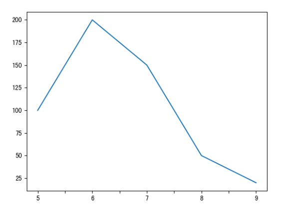
s.plot()以s的索引为横坐标,s的各元素为纵坐标画折线图
s = pd.Series([100, 200, 150, 50, 20], index=list('56789'))
s.plot()
plt.show()
例:正弦曲线
x = np.arange(0, 2*np.pi, 0.1)  # 0-2pai的数,间隔为0.1
y = np.sin(x)  # y=sin(x)
data = pd.Series(data=y, index=x)
data.plot()
plt.show()
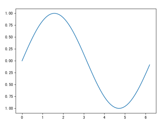
因为这里给的x值足够多,所以看起来是曲线
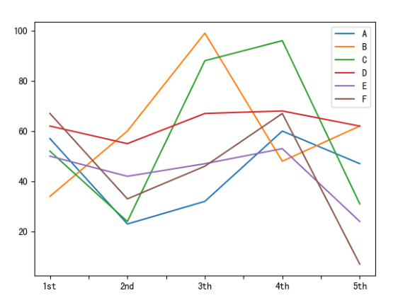
df.plot()每一列数据画一根折线,还是以行索引为横坐标,数据值为纵坐标
如果想每一行数据画一根折线,就先转置再画:df.T.plot()(使用较少)
data = np.random.randint(0, 100, size=(5, 6))
index = ['1st', '2nd', '3th', '4th', '5th']
columns = list('ABCDEF')
df = pd.DataFrame(data=data, index=index, columns=columns)
print(df)
df.plot()
plt.show()
      A   B   C   D   E   F
1st  57  34  52  62  50  67
2nd  23  60  24  55  42  33
3th  32  99  88  67  47  46
4th  60  48  96  68  53  67
5th  47  62  31  62  24   7
条形图/柱状图
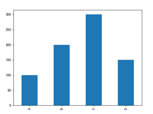
s.plot(kind='bar')或s.plot.bar(),s的索引为横坐标,s的各元素为纵坐标
s = pd.Series(data=[100, 200, 300, 150], index=list('ABCD'))
s.plot.bar()
plt.show()
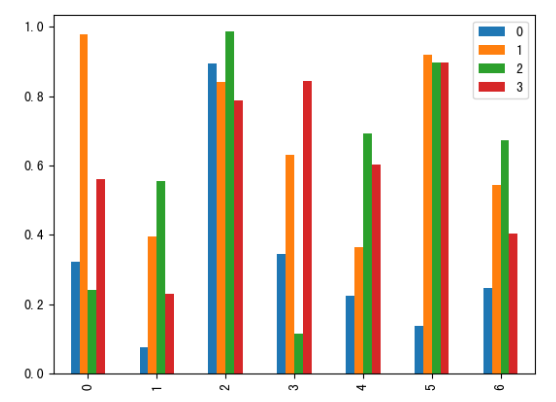
df.plot(kind='bar')或df.plot.bar(),横坐标为行索引,每个数据都有一个柱子
df = pd.DataFrame(data=np.random.rand(7, 4))
df.plot(kind='bar')
plt.show()
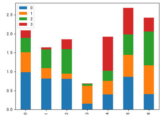
在绘图函数中添加参数stacked=True可以使柱状图堆叠
df = pd.DataFrame(data=np.random.rand(7, 4))
df.plot.bar(stacked=True)
plt.show()
将参数kind='bar'改成kind='barh'或者使用plot.barh()可以画水平的柱状图
s = pd.Series(data=[100, 200, 300, 150], index=list('ABCD'))
s.plot.barh()
plt.show()
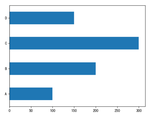
一般可以把水平的称为条形图,竖直的称为柱状图
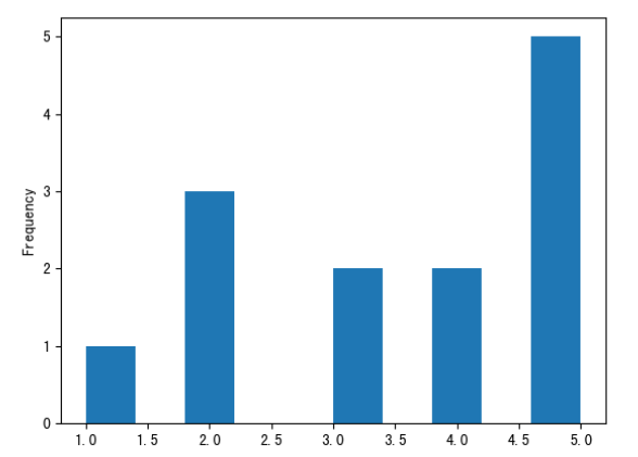
直方图/kde图
直方图中柱高表示数据的频数(出现次数),柱宽表示各组数据的组距
s.plot(kind='hist')或s.plot.hist()
可传入参数:
-
bins=n设置柱子的个数上限为n,n越大则柱宽越小,数据分组越细致 -
density=True将频数转换为概率
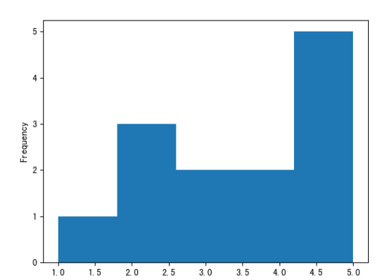
s = pd.Series([1, 2, 2, 2, 3, 3, 4, 4, 5, 5, 5, 5, 5])
s.plot.hist()
plt.show()
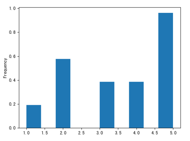
s = pd.Series([1, 2, 2, 2, 3, 3, 4, 4, 5, 5, 5, 5, 5])
s.plot(kind='hist', bins=5)
plt.show()
s = pd.Series([1, 2, 2, 2, 3, 3, 4, 4, 5, 5, 5, 5, 5])
s.plot.hist(density=True)
plt.show()
如果想将一个df的每列都画一个直方图,可以使用参数subplots=True
df = pd.DataFrame(data=np.random.rand(4,2), index=list('abcd'), columns=['A', 'B'])
df.plot(kind='hist', subplots=True)
plt.show()
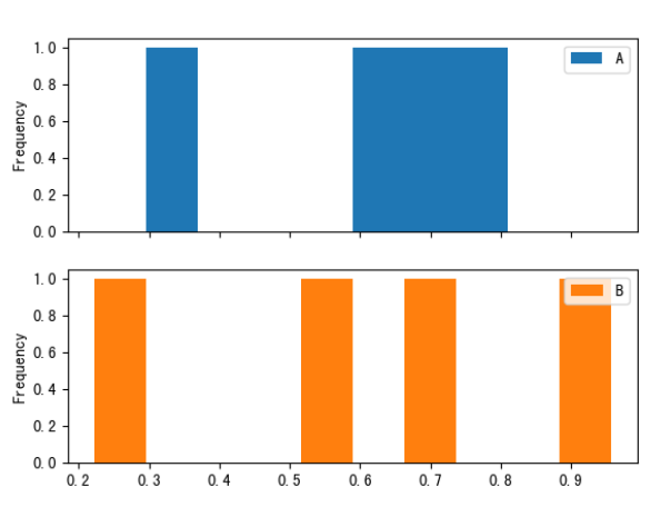
此参数可适用于各种原本用于series的画图函数
kde图:核密度估计,用于弥补直方图中由于bins参数设置不合理 导致的精度缺失问题
s.plot(kind='kde')或s.plot.kde()
s = pd.Series([1, 2, 2, 2, 3, 3, 4, 4, 5, 5, 5, 5, 5])
s.plot(kind='kde')
plt.show()
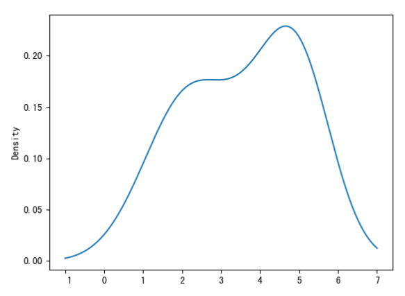
可以看到是一条曲线,更精确显示每个值的概率和变化趋势
一般情况下它与直方图联用(画在一起):
s = pd.Series([1, 2, 2, 2, 3, 3, 4, 4, 5, 5, 5, 5, 5])
s.plot(kind='hist', density=True)
s.plot.kde()
plt.show()
饼图
用于显示各项数据占总数的比例
s.plot(kind='pie')或s.plot.pie()
s = pd.Series([1, 3, 4], index=list('ABC'))
s.plot(kind='pie')
plt.show()
可以看到数据的总和为1+3+4=8,A部分占比即为1/8、B部分占比即为3/8、C部分占比即为4/8
可以设置参数autopct='%.1f%%使显示每部分的占比百分数(.1f%就是保留一位小数)
s = pd.Series([1, 3, 4], index=list('ABC'))
s.plot.pie(autopct='%.1f%%')
plt.show()
更复杂的例子:
df = pd.DataFrame(data=np.random.rand(4,2), index=list('abcd'), columns=['A', 'B'])
df.plot.pie(subplots=True, figsize=(8, 4), autopct='%.2f%%')  # 定义尺寸和保留小数
plt.show()
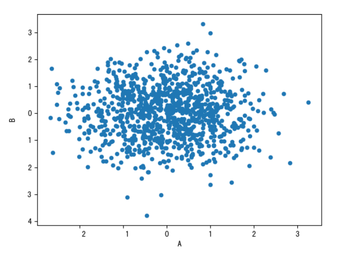
散点图
散点图一般用于描述两列数据的关系
df.plot(kind='scatter', x='列名1', y='列名2')或df.plot.scatter(x='列名1', y='列名2') 指定X/Y轴分别是哪列
df = pd.DataFrame(data=np.random.normal(size=(1000, 2)), columns=['A', 'B'])
df.plot.scatter(x='A', y='B')
plt.show()
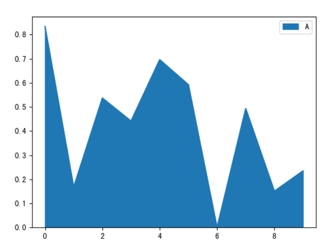
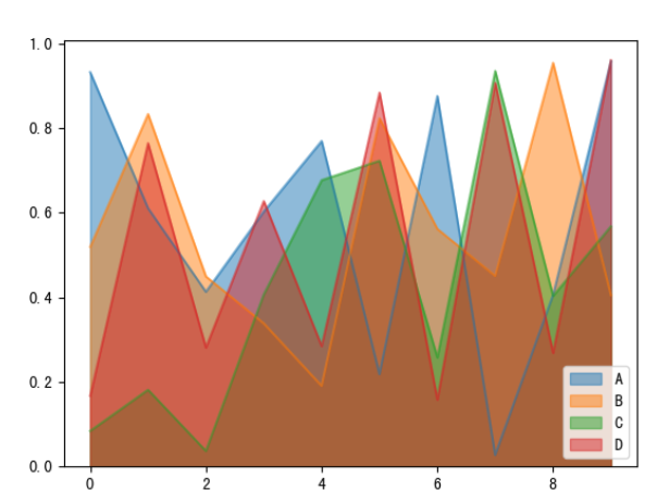
面积图
s.plot(kind='area')或s.plot.area()
df.plot(kind='area')或df.plot.area()
和折线图类似,只不过把折线下边的空间染色了
df = pd.DataFrame(data=np.random.rand(10, 4), columns=list('ABCD'))
df[['A']].plot.area()
plt.show()
df = pd.DataFrame(data=np.random.rand(10, 4), columns=list('ABCD'))
df.plot(kind='area')
plt.show()
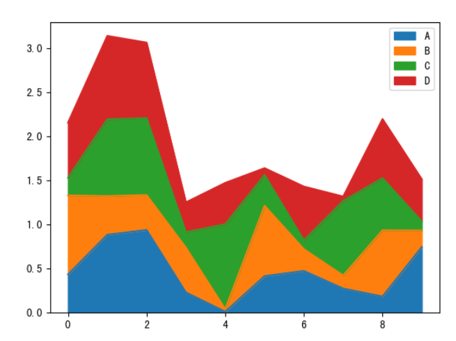
可设置参数stacked=False禁止堆叠
df = pd.DataFrame(data=np.random.rand(10, 4), columns=list('ABCD'))
df.plot(kind='area', stacked=False)
plt.show()
箱型图
s.plot(kind='box')或s.plot.box()
df.plot(kind='box')或df.plot.box()
df = pd.DataFrame(data=np.random.rand(10, 4), columns=list('ABCD'))
df[['A']].plot.box()
df.plot(kind='box')
plt.show()
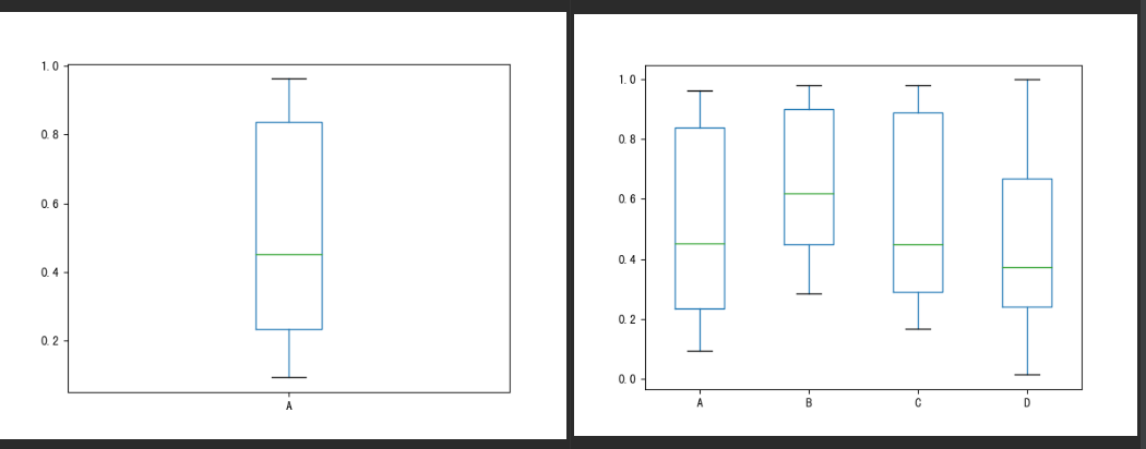
箱型图中各部分含义:
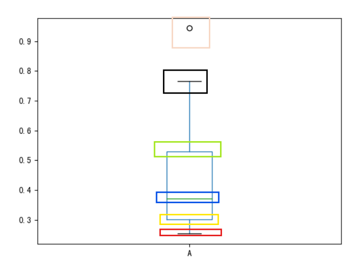
从上到下依次为:
-
离群值(异常值),表示为空心圆点
-
(排除离群值后的)最大值
-
75%分位点
-
50%分位点
-
25%分位点
-
(排除离群值后的)最小值
案例
条形图
读取文件tips.csv,day列为星期几,其余列索引是聚会规模,数据是某天某规模的聚会有几次
tips = pd.read_csv("data/pandas/tips.csv")
print(tips)
    day  1   2   3   4  5  6
0   Fri  1  16   1   1  0  0
1  Stat  2  53  18  13  1  0
2   Sun  0  39  15  18  3  1
3  Thur  1  48   4   5  1  3
任务:
-
把day作为行索引
tips = tips.set_index('day')1 2 3 4 5 6 day Fri 1 16 1 1 0 0 Stat 2 53 18 13 1 0 Sun 0 39 15 18 3 1 Thur 1 48 4 5 1 3 -
求每天的聚会规模,即每天共有多少次聚会
day_sum = tips.sum(axis=1) # 对行求和day Fri 19 Stat 87 Sun 76 Thur 62 dtype: int64 -
每天各种规模的聚会占比,即每个数据除以总数
new_tips = tips.div(day_sum, axis=0) # 用tips的每列去除day_sum1 2 3 4 5 6 day Fri 0.052632 0.842105 0.052632 0.052632 0.000000 0.000000 Stat 0.022989 0.609195 0.206897 0.149425 0.011494 0.000000 Sun 0.000000 0.513158 0.197368 0.236842 0.039474 0.013158 Thur 0.016129 0.774194 0.064516 0.080645 0.016129 0.048387 -
画图
new_tips.plot.bar()
plt.show()
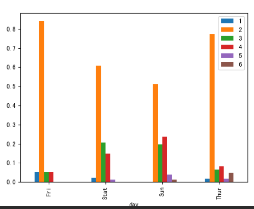
代码汇总:
tips = pd.read_csv("data/pandas/tips.csv")
tips = tips.set_index('day')
day_sum = tips.sum(axis=1)  # 对行求和
new_tips = tips.div(day_sum, axis=0)  # 用tips的每列去除day_sum
new_tips.plot.bar()
plt.show()
综合案例1
读取数据AAPL.csv,是关于一支股票的信息
data = pd.read_csv('data/pandas/AAPL.csv')
# data.sample(n=5)
            Date       Open       High  ...      Close  Adj Close     Volume
257   1981-12-21   0.392857   0.392857  ...   0.390625   0.320780   14100800
7634  2011-03-18  48.161430  48.314285  ...  47.238571  42.498463  188303500
6972  2008-08-01  22.842857  22.855715  ...  22.379999  20.134302  136159800
7435  2010-06-04  36.887142  37.414288  ...  36.565716  32.896561  189576100
3065  1993-01-28   2.142857   2.151786  ...   2.138393   1.852755   46009600
# data.dtypes
Date          object
Open         float64
High         float64
Low          float64
Close        float64
Adj Close    float64
Volume         int64
dtype: object
-
将date列转为时间数据类型,并设为行索引
data = pd.read_csv('data/pandas/AAPL.csv')
data['Date'] = pd.to_datetime(data['Date'])
new_data = data.set_index(keys='Date')
# new_data.sample(n=5) Open High Low Close Adj Close Volume Date 1995-01-09 1.486607 1.495536 1.464286 1.471539 1.308915 68521600 2000-01-27 3.886161 4.035714 3.821429 3.928571 3.534363 85036000 2007-07-13 19.290001 19.692858 19.217142 19.675714 17.701376 226901500 1990-11-12 1.267857 1.312500 1.258929 1.294643 1.097993 36262800 2009-10-22 29.242857 29.692858 28.930000 29.314285 26.372772 197848000 -
绘制
Adj Close的变化趋势图:因为数据足够多,直接绘制散点图就能连成线new_data['Adj Close'].plot() plt.show()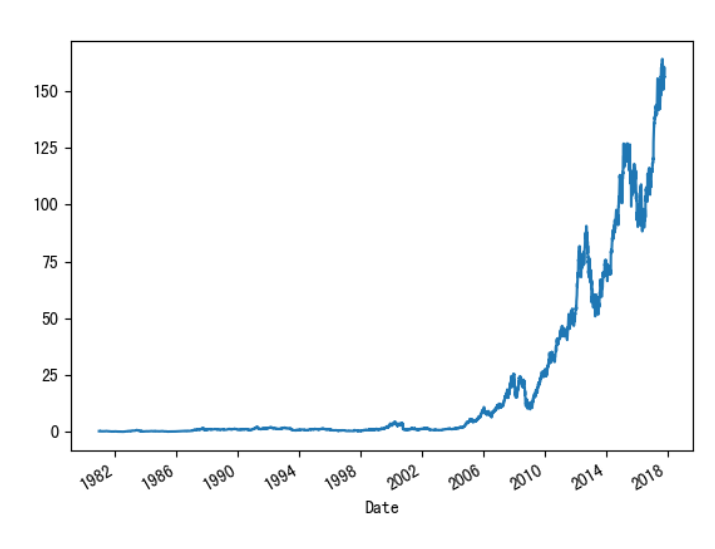
代码汇总:
import pandas as pd
import matplotlib.pyplot as plt
data = pd.read_csv('data/pandas/AAPL.csv')
data['Date'] = pd.to_datetime(data['Date'])
new_data = data.set_index(keys='Date')
new_data['Adj Close'].plot()
plt.show()
综合案例2
美国人口数据分析:读取数据–
-
state-abbrevs.csv每个州的缩写名称 -
state-areas.csv每个州的面积 -
state-population.csv每个州不同年份18岁以下的人数、总人数
abb = pd.read_csv('data/pandas/state-abbrevs.csv')
areas = pd.read_csv('data/pandas/state-areas.csv')
pop = pd.read_csv('data/pandas/state-population.csv')
# abb.sample(n=5)
            state abbreviation
12          Idaho           ID
42      Tennessee           TN
31         Oregon           OR
24     New Jersey           NJ
23  New Hampshire           NH
# areas.sample(n=5)
             state  area (sq. mi)
21        Michigan          96810
14            Iowa          56276
32  North Carolina          53821
1           Alaska         656425
29      New Jersey           8722
# pop.sample(n=5)
     state/region     ages  year  population
1079           MI  under18  2002   2584310.0
362            DE    total  2004    830803.0
1030           MA    total  2001   6397634.0
2352           WI  under18  1990   1302869.0
847            KY  under18  2006   1011295.0
-
合并pop和abb,保留所有信息(不去除缺失值),并去除合并重复的
abbreviation列pop_abb = pop.merge(abb, left_on='state/region', right_on='abbreviation', how='outer') # 使用外合并,不去除缺失值 pop_abb.drop(columns='abbreviation', inplace=True) # 更改原数据# pop_abb.head() state/region ages year population state 0 AL under18 2012 1117489.0 Alabama 1 AL total 2012 4817528.0 Alabama 2 AL under18 2010 1130966.0 Alabama 3 AL total 2010 4785570.0 Alabama 4 AL under18 2011 1125763.0 Alabama -
查看数据中哪列存在缺失值,并查看缺失数据的行
print(pop_abb.isnull().any())state/region False ages False year False population True state True dtype: bool可以看到
population和state列存在缺失值cond = pop_abb.isnull().any(axis=1) # 存在空值的行 print(pop_abb.loc[cond])state/region ages year population state 2448 PR under18 1990 NaN NaN 2449 PR total 1990 NaN NaN ... ... ... ... ... ... 2542 USA under18 2012 73708179.0 NaN 2543 USA total 2012 313873685.0 NaN [96 rows x 5 columns] -
找到有哪些
state/region的state列值为NaN:先找到state列值为NaN的行,再提取这些行state/region列的值,最后用unique去重cond = pop_abb['state'].isnull() print(pop_abb.loc[cond]['state/region'].unique()) # ['PR' 'USA'] -
填充state这列上所有的空值
-
state/region列值为”PR”的,填充成”Puerto Rico” -
USA -> United State
is_PR = pop_abb['state/region'] == 'PR'
is_USA = pop_abb['state/region'] == 'USA'
pop_abb['state'][is_PR] = "Puerto Rico"
pop_abb['state'][is_USA] = "United State"
state/region ages year population state 2448 PR under18 1990 NaN Puerto Rico 2449 PR total 1990 NaN Puerto Rico 2450 PR total 1991 NaN Puerto Rico 2451 PR under18 1991 NaN Puerto Rico 2452 PR total 1993 NaN Puerto Rico -
-
合并面积数据areas,使用左合并保留
pop_abb的所有值pop_abb_areas = pop_abb.merge(areas, how='left')state/region ages year population state area (sq. mi) 0 AL under18 2012 1117489.0 Alabama 52423.0 1 AL total 2012 4817528.0 Alabama 52423.0 2 AL under18 2010 1130966.0 Alabama 52423.0 3 AL total 2010 4785570.0 Alabama 52423.0 4 AL under18 2011 1125763.0 Alabama 52423.0 -
找出area列出现空值的state,并去除含缺失数据的行
cond = pop_abb_areas['area (sq. mi)'].isnull() print(pop_abb_areas['state'][cond].unique()) # ['United State'] cond = pop_abb_areas.notnull().all(axis=1) # 获取所有非空的行 pop_abb_areas = pop_abb_areas.loc[cond] -
找出2010年总人口数据,并以state作为新的行索引
pop_2010 = pop_abb_areas.query('year==2010 and ages=="total"')
pop_2010.set_index('state', inplace=True)
state/region ages year population area (sq. mi) state Alabama AL total 2010 4785570.0 52423.0 Alaska AK total 2010 713868.0 656425.0 Arizona AZ total 2010 6408790.0 114006.0 Arkansas AR total 2010 2922280.0 53182.0 California CA total 2010 37333601.0 163707.0 -
计算人口密度density=population/area
pop_2010['density'] = pop_2010['population'] / pop_2010['area (sq. mi)']state/region ages year population area (sq. mi) density state Alabama AL total 2010 4785570.0 52423.0 91.287603 Alaska AK total 2010 713868.0 656425.0 1.087509 Arizona AZ total 2010 6408790.0 114006.0 56.214497 Arkansas AR total 2010 2922280.0 53182.0 54.948667 California CA total 2010 37333601.0 163707.0 228.051342 -
排序,找出人口密度最高/最低的五个州
top_5 = pop_2010.sort_values('density', ascending=False).head(5)
last_5 = pop_2010.sort_values('density', ascending=True).head(5)
state/region ages ... area (sq. mi) density state ... District of Columbia DC total ... 68.0 8898.897059 Puerto Rico PR total ... 3515.0 1058.665149 New Jersey NJ total ... 8722.0 1009.253268 Rhode Island RI total ... 1545.0 681.339159 Connecticut CT total ... 5544.0 645.600649 state/region ages year population area (sq. mi) density state Alaska AK total 2010 713868.0 656425.0 1.087509 Wyoming WY total 2010 564222.0 97818.0 5.768079 Montana MT total 2010 990527.0 147046.0 6.736171 North Dakota ND total 2010 674344.0 70704.0 9.537565 South Dakota SD total 2010 816211.0 77121.0 10.583512
代码汇总:
import pandas as pd
# 读取数据
abb = pd.read_csv('data/pandas/state-abbrevs.csv')
areas = pd.read_csv('data/pandas/state-areas.csv')
pop = pd.read_csv('data/pandas/state-population.csv')
# 合并pop和abb
pop_abb = pop.merge(abb, left_on='state/region', right_on='abbreviation', how='outer')  # 使用外合并,不去除缺失值
# 去除合并重复的abbreviation列
pop_abb.drop(columns='abbreviation', inplace=True)  # inplace=True设定更改原数据
# 填充state列所有的空值
is_PR = pop_abb['state/region'] == 'PR'
is_USA = pop_abb['state/region'] == 'USA'
pop_abb['state'][is_PR] = "Puerto Rico"
pop_abb['state'][is_USA] = "United State"
# 合并面积数据
pop_abb_areas = pop_abb.merge(areas, how='left')  # 使用左合并保留pop_abb的所有值
# 去除含缺失数据的行
cond = pop_abb_areas.notnull().all(axis=1)  # 获取所有非空行的索引
pop_abb_areas = pop_abb_areas.loc[cond]  # 保留非空的行
# 找出2010年总人口数据
pop_2010 = pop_abb_areas.query('year==2010 and ages=="total"')
# 以state作为新的行索引
pop_2010.set_index('state', inplace=True)
# 计算人口密度density
pop_2010['density'] = pop_2010['population'] / pop_2010['area (sq. mi)']
# 排序
top_5 = pop_2010.sort_values('density', ascending=False).head(5)  # 从高到低(降序)
last_5 = pop_2010.sort_values('density', ascending=True).head(5)  # 从低到高(升序)