GSE157827数据集练习

other-other

2025.12.17-2025.12.31研究进展

跟着教程做复现

参考教程：复现2：AD与Normal细胞类型水平的差异基因挖掘(snRNA-seq)

构建Seurat对象

下载计数矩阵

cd /public/home/GENE_proc/wth/GSE157827/raw_data/raw_mtx_gz/
wget https://ftp.ncbi.nlm.nih.gov/geo/series/GSE157nnn/GSE157827/suppl/GSE157827_RAW.tar
tar -xvf GSE157827_RAW.tar
rm GSE157827_RAW.tar

使用Read10X直接构建Seurat对象

library(Seurat)
library(tidyverse)
root_dir <- '/public/home/GENE_proc/wth/GSE157827/raw_data/raw_mtx_gz/'
fs <- list.files(root_dir, '^GSM')
samples <- str_split(fs, '_', simplify = T)[, 1]
# 批量将文件名改为 Read10X()函数能够识别的名字
lapply(unique(samples), function(x){
    y <- fs[grepl(x, fs)]
    folder <- paste0(root_dir, paste(str_split(y[1], '_', simplify = T)[, 1:2], collapse = "_"))
    dir.create(folder,recursive = T)
    # 为每个样本创建子文件夹
    file.rename(paste0(root_dir, y[1]), file.path(folder, "barcodes.tsv.gz"))
    # 重命名文件，并移动到相应的子文件夹里
    file.rename(paste0(root_dir, y[2]), file.path(folder, "features.tsv.gz"))
    file.rename(paste0(root_dir, y[3]), file.path(folder, "matrix.mtx.gz"))
})
samples <- list.files(root_dir, '^GSM')
dir <- file.path(root_dir, samples)
names(dir) <- samples
# 创建Seurat对象
counts <- Read10X(data.dir = dir)
scRNA <- CreateSeuratObject(counts)

> dim(scRNA)  # 查看基因数和细胞总数
[1]  33538 179392
> table(scRNA@meta.data$orig.ident)  # 查看每个样本的细胞数
GSM4775561 GSM4775562 GSM4775563 GSM4775564 GSM4775565 GSM4775566 GSM4775567 
      6243      15357       6166      12362       2990       2654      10229 
GSM4775568 GSM4775569 GSM4775570 GSM4775571 GSM4775572 GSM4775573 GSM4775574 
     16156       1829       3794       9208       8472       6327       6483 
GSM4775575 GSM4775576 GSM4775577 GSM4775578 GSM4775579 GSM4775580 GSM4775581 
      3576      15692      10983       8416       6348      14491      11616 
> colnames(scRNA@meta.data)
[1] "orig.ident"   "nCount_RNA"   "nFeature_RNA"

metadata细节整理

metadata.xlsx：GSM号到样本号（AD1/NC1这种）的映射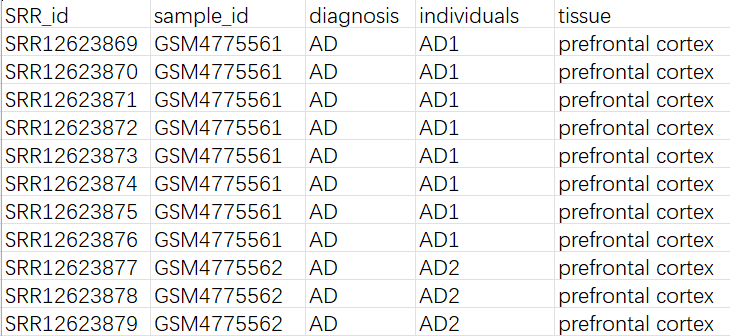
sample_info.xlsx：每个样本的年龄性别等诊断信息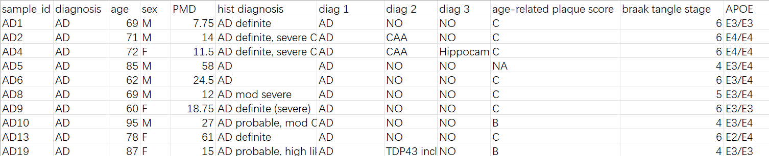

library(readxl)
# 读入并整理两个xlsx
meta_map <- read_xlsx("/public/home/GENE_proc/wth/GSE157827/raw_data/metadata/metadata.xlsx")
names(meta_map) <- make.names(names(meta_map))
meta_map <- meta_map %>%
  transmute(
    GSM       = as.character(sample_id),
    sample_id = as.character(individuals),
    group     = as.character(diagnosis),
    tissue    = as.character(tissue)
  ) %>%
  distinct()
sample_info <- read_xlsx("/public/home/GENE_proc/wth/GSE157827/raw_data/metadata/sample_info.xlsx")
names(sample_info) <- make.names(names(sample_info))
sample_info <- sample_info %>%
  mutate(sample_id = as.character(sample_id)) %>%
  select(-any_of("diagnosis"))
# 从Seurat取出每个细胞对应的GSM，并做两次join
cell_meta <- scRNA@meta.data %>%
  rownames_to_column("cell") %>%
  mutate(GSM = as.character(orig.ident))
cell_meta2 <- cell_meta %>%
  left_join(meta_map,    by = "GSM") %>%
  left_join(sample_info, by = "sample_id")
# 检查是否有映射失败
n_unmapped <- sum(is.na(cell_meta2$sample_id))
n_unmapped
# 添加metadata
new_cols <- setdiff(names(cell_meta2), names(scRNA@meta.data))
meta_to_add <- cell_meta2 %>%
  select(cell, all_of(new_cols)) %>%
  column_to_rownames("cell")
scRNA <- AddMetaData(scRNA, metadata = meta_to_add)
# orig.ident用AD1/NC1，group用AD/NC，并设置排序
scRNA$orig.ident <- scRNA$sample_id
scRNA$group <- factor(scRNA$group, levels = c("NC", "AD"))
sample_levels <- unique(as.character(scRNA$orig.ident))
num_part <- as.numeric(str_extract(sample_levels, "\\d+"))
grp_part <- substr(sample_levels, 1, 2)
ord <- order(match(grp_part, c("NC", "AD")), num_part)
scRNA$orig.ident <- factor(scRNA$orig.ident, levels = sample_levels[ord])

保存为rds对象

saveRDS(
    scRNA, 
    file = file.path("/public/home/GENE_proc/wth/GSE157827/data/", "GSE157827.rds"), 
    compress = "xz"
)

抽取1/3到本地电脑作测试

set.seed(20251220)
prop_keep <- 1/3
cells_keep <- scRNA@meta.data %>%
  rownames_to_column("cell") %>%
  group_by(orig.ident) %>%
  slice_sample(prop = prop_keep) %>%
  pull(cell)
scRNA_smaller <- subset(scRNA, cells = cells_keep)
# 检查抽样结果
print(ncol(scRNA)); print(ncol(scRNA_smaller))  # 179392  59791
print(table(scRNA_smaller$group))
print(table(scRNA_smaller$orig.ident, scRNA_smaller$group))
# 保存
saveRDS(
    scRNA_smaller, 
    file = file.path("/public/home/GENE_proc/wth/GSE157827/data/", "GSE157827_smaller.rds"), 
    compress = "xz"
)

看一看结果

scRNA <- readRDS("C:\\Users\\17185\\Desktop\\hERV_calc\\GSE157827\\data\\GSE157827_smaller.rds")
# scRNA <- readRDS("/public/home/GENE_proc/wth/GSE157827/data/GSE157827.rds")
res_dir <- "C:\\Users\\17185\\Desktop\\hERV_calc\\GSE157827\\res"
# res_dir <- "/public/home/GENE_proc/wth/GSE157827/教程复现/res/"

> scRNA
An object of class Seurat 
33538 features across 59791 samples within 1 assay 
Active assay: RNA (33538 features, 0 variable features)
 1 layer present: counts

跟着教程做复现_GSE157827_3

质控

library(Seurat)
library(tidyverse)
library(patchwork)
library(ggVennDiagram)
library(Matrix)
library(ggbreak)

注：后续的结果输出/图片都是使用完整数据的

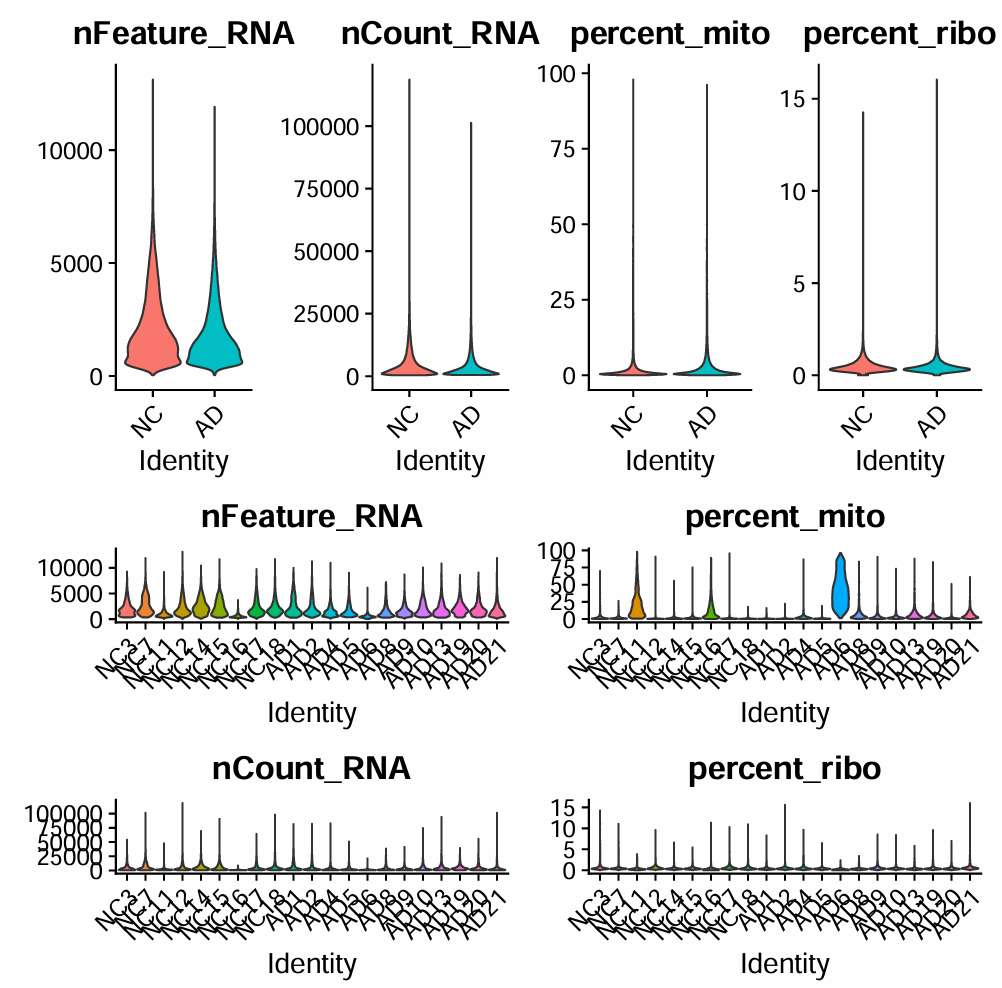
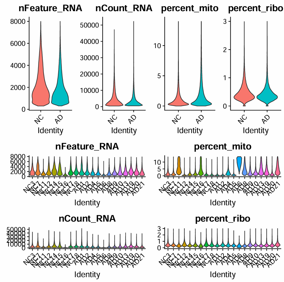
过滤前的各项指标

# 基因数/UMI数
feats <- c("nFeature_RNA", "nCount_RNA")
p_filt_b_1 <- VlnPlot(
  scRNA, features = feats,
  pt.size = 0,
  ncol = 2,
  group.by = "group"  # 按AD/NC分组看分布
) + NoLegend()
p_filt_b_2 <- VlnPlot(
  scRNA, features = feats,
  pt.size = 0,
  ncol = 1,
  group.by = "orig.ident"  # 按样本(AD1/NC1...)看分布
) + NoLegend()
# 线粒体/核糖体比例
mito_genes <- rownames(scRNA)[grep("^MT-", rownames(scRNA))]  # 线粒体基因：通常以"MT-"开头
scRNA <- PercentageFeatureSet(scRNA, pattern = "^MT-", col.name = "percent_mito")  # 每个细胞中，线粒体基因UMI占比
ribo_genes <- rownames(scRNA)[grep("^Rp[sl]", rownames(scRNA), ignore.case = TRUE)]  # 核糖体基因：通常以RPL或RPS开头
scRNA <- PercentageFeatureSet(scRNA, pattern = "^RP[SL]", col.name = "percent_ribo")  # 每个细胞中，核糖体基因UMI占比
feats <- c("percent_mito", "percent_ribo")
p_filt_b_3 <- VlnPlot(
  scRNA, features = feats, 
  pt.size = 0, 
  ncol = 2,
  group.by = "group"  # 按AD/NC分组看分布
) + NoLegend()
p_filt_b_4 <- VlnPlot(
  scRNA, features = feats, 
  pt.size = 0, 
  ncol = 1,
  group.by = "orig.ident"  # 按样本看分布
) + NoLegend()
# 拼图展示
pdf(file.path(res_dir, "before_filter.pdf"))
p <- (p_filt_b_1 / p_filt_b_2) | (p_filt_b_3 / p_filt_b_4)
print(p)
dev.off()

> fivenum(scRNA@meta.data$percent_mito)
[1]  0.0000000  0.4171011  0.9939049  2.5860344 97.8759558
> fivenum(scRNA@meta.data$percent_ribo)
[1]  0.0000000  0.2645503  0.3795066  0.5625879 16.0344828

对应min / Q1 / median / Q3 / max这5个指标，快速了解分布范围，大概看一下阈值怎么取

跟着教程做复现_GSE157827_4

和之前的教程比起来，他多了一个核糖体基因基因比例，这个指标也可能提示污染或技术噪声

确定过滤阈值

细胞阈值：

# 设置阈值
retained_c_umi_low  <- scRNA$nFeature_RNA > 300
retained_c_umi_high <- scRNA$nFeature_RNA < 8000
retained_c_mito     <- scRNA$percent_mito < 14
retained_c_ribo     <- scRNA$percent_ribo < 3
keep_cells <- retained_c_mito & retained_c_ribo & retained_c_umi_low & retained_c_umi_high
# 用Venn图看看是哪个过滤条件剔除了细胞
umi_low  <- Cells(scRNA)[!retained_c_umi_low]
umi_high <- Cells(scRNA)[!retained_c_umi_high]
mito     <- Cells(scRNA)[!retained_c_mito]
ribo     <- Cells(scRNA)[!retained_c_ribo]
veen_eles <- list(
  `Filt_low_umi\n(300)`   = umi_low,
  `Filt_high_umi\n(8000)` = umi_high,
  `Filt_high_mito\n(14%)` = mito,
  `Filt_high_ribo\n(3%)`  = ribo
)
pdf(file.path(res_dir, "cell_filter.pdf"), width = 12, height = 8)
p <- ggVennDiagram(veen_eles, set_size = 4) +
  scale_fill_gradient(low = "#ffffb2", high = "#f03b20")
print(p)
dev.off()

> table(keep_cells)  # 看看最后保留/剔除多少细胞
keep_cells
 FALSE   TRUE 
  9876 169516 
> table(scRNA$group[keep_cells])  # 看看保留下来的细胞在AD/NC里各多少（检查过滤是否对某组特别“偏心”）
   NC    AD 
79036 90480 

跟着教程做复现_GSE157827_5

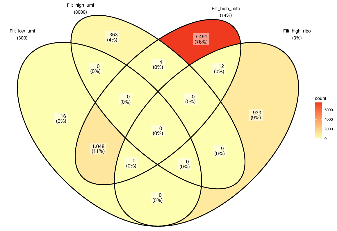
如果Filt_low_umi单独占很大：说明很多细胞信息量太少
如果Filt_high_mito/Filt_high_ribo占很大（图中情况）：说明样本可能有较多“质量差/污染/应激”的核
大量重叠（比较常见）：表示同一批坏细胞同时表现出多种坏指标

基因阈值：按“在多少细胞里出现过”过滤基因，去掉极低频基因（例如只在极少数细胞里出现一次的噪声）

减少噪声，加快后续计算速度

counts <- GetAssayData(scRNA, assay = "RNA", slot = "counts")
feature_rowsum <- Matrix::rowSums(counts > 0)  # 每个基因在多少个细胞里出现过
# 只保留“至少在0.5%细胞里表达过”的基因
retained_f_low <- feature_rowsum > ncol(scRNA) * 0.005
# rankplot辅助看阈值
rankplot <- data.frame(
  feature_count = sort(feature_rowsum),
  gene = names(sort(feature_rowsum)),
  Rank = 1:length(feature_rowsum)
)
pdf(file.path(res_dir, "gene_filter.pdf"), width = 12, height = 8)
p <- ggplot(rankplot, aes(x = Rank, y = feature_count)) +
  geom_point() +
  scale_y_break(c(10000, 100000)) +  # 断轴，避免极高表达基因把图压扁
  geom_hline(
    yintercept = ncol(scRNA) * 0.005, 
    color = "red"
  ) +
  geom_text(
    x = 10000, y = 4000, size = 5,
    label = "Feature cutoff : ncol(scRNA)*0.5%"
  )
print(p)
dev.off()

> table(retained_f_low)
retained_f_low
FALSE  TRUE 
16262 17276 

跟着教程做复现_GSE157827_6

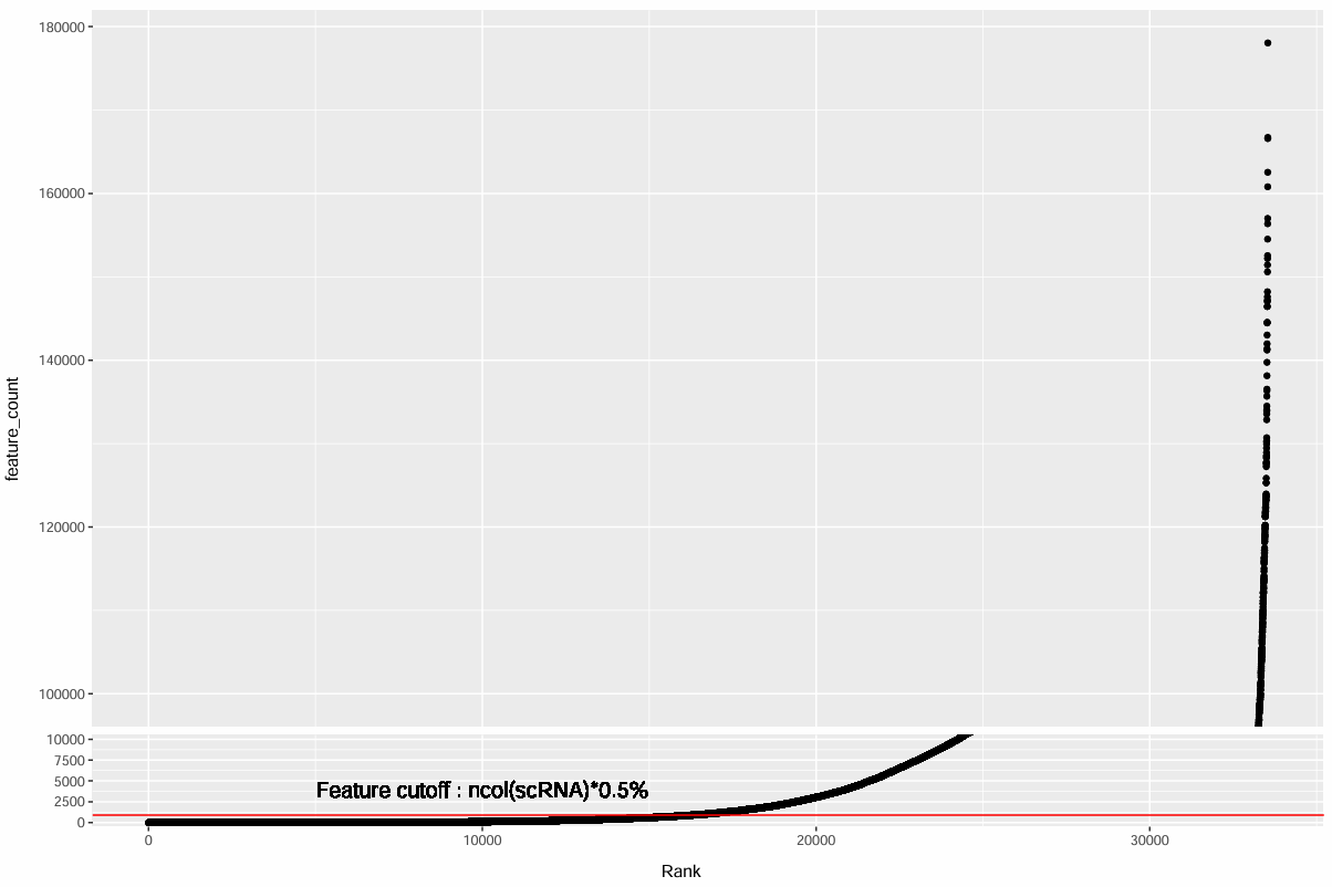
红线就是阈值（在多少个细胞里表达过）
红线以下的点 = 低频基因（被过滤掉）
只要确认红线切的位置“在低频尾巴”而不是切到主体即可

过滤

scRNA_filt <- scRNA[retained_f_low, keep_cells]
# 过滤后的各项指标
feats <- c("nFeature_RNA", "nCount_RNA")
p_filt_a_1 <- VlnPlot(
  scRNA_filt, features = feats, 
  pt.size = 0, ncol = 2,
  group.by = "group"
) + NoLegend()
p_filt_a_2 <- VlnPlot(
  scRNA_filt, features = feats, 
  pt.size = 0, ncol = 1,
  group.by = "orig.ident"
) + NoLegend()
feats <- c("percent_mito", "percent_ribo")
p_filt_a_3 <- VlnPlot(
  scRNA_filt, features = feats, 
  pt.size = 0, ncol = 2,
  group.by = "group"
) + NoLegend()
p_filt_a_4 <- VlnPlot(
  scRNA_filt, features = feats, 
  pt.size = 0, ncol = 1,
  group.by = "orig.ident"
) + NoLegend()
pdf(file.path(res_dir, "after_filter.pdf"))
p <- (p_filt_a_1 / p_filt_a_2) | (p_filt_a_3 / p_filt_a_4)
print(p)
dev.off()

> dim(scRNA_filt)  # 过滤后的基因数x细胞数
[1]  17276 169516
> table(scRNA_filt$group)  # 过滤后AD/NC细胞数
   NC    AD 
79036 90480 

跟着教程做复现_GSE157827_8

dim(scRNA_filt)：细胞数会下降、基因数也会下降
nFeature_RNA的下尾被“抬高”（低质量细胞被清掉）
percent_mito/percent_ribo的高尾被砍掉（异常核比例下降）

# 保存过滤后的对象
saveRDS(
    scRNA_filt, 
    file = file.path("C:\\Users\\17185\\Desktop\\hERV_calc\\GSE157827\\data", "GSE157827_smaller_filt.rds"), 
    compress = "xz"
)
# saveRDS(
#     scRNA_filt, 
#     file = file.path("/public/home/GENE_proc/wth/GSE157827/data/", "GSE157827_filt.rds"), 
#     compress = "xz"
# )

数据预处理

library(Seurat)
library(tidyverse)
library(patchwork)
library(clustree)
# library(future)
# # future设置（如果后续报错可以不执行这段）
# plan("multisession", workers = 4)
# options(future.globals.maxSize = 20000 * 1024^2)

scRNA <- readRDS("C:\\Users\\17185\\Desktop\\hERV_calc\\GSE157827\\data\\GSE157827_smaller_filt.rds")
# scRNA <- readRDS("/public/home/GENE_proc/wth/GSE157827/data/GSE157827_filt.rds")
res_dir <- "C:\\Users\\17185\\Desktop\\hERV_calc\\GSE157827\\res"
# res_dir <- "/public/home/GENE_proc/wth/GSE157827/教程复现/res/"

由于数据量比较大，ScaleData函数比较耗时，尤其是加上回归参数。可使用future包的plan函数设置线程数

推荐使用四个线程，此外如果在FindIntegrationAnchors步骤使用报错，设置options(future.globals.maxSize = 1000 * 1024^2)即可

# NormalizeData
scRNA <- NormalizeData(
  scRNA,
  normalization.method = "LogNormalize",
  scale.factor = 10000
)
# FindVariableFeatures
scRNA <- FindVariableFeatures(
  scRNA,
  selection.method = "vst",
  nfeatures = 2000
)
# ScaleData
scRNA <- ScaleData(
  scRNA,
  features = VariableFeatures(scRNA),
  vars.to.regress = c("nFeature_RNA", "percent_mito")    # 根据教程，回归了nFeature_RNA和percent_mito
)
# PCA
scRNA <- RunPCA(scRNA, features = VariableFeatures(scRNA))
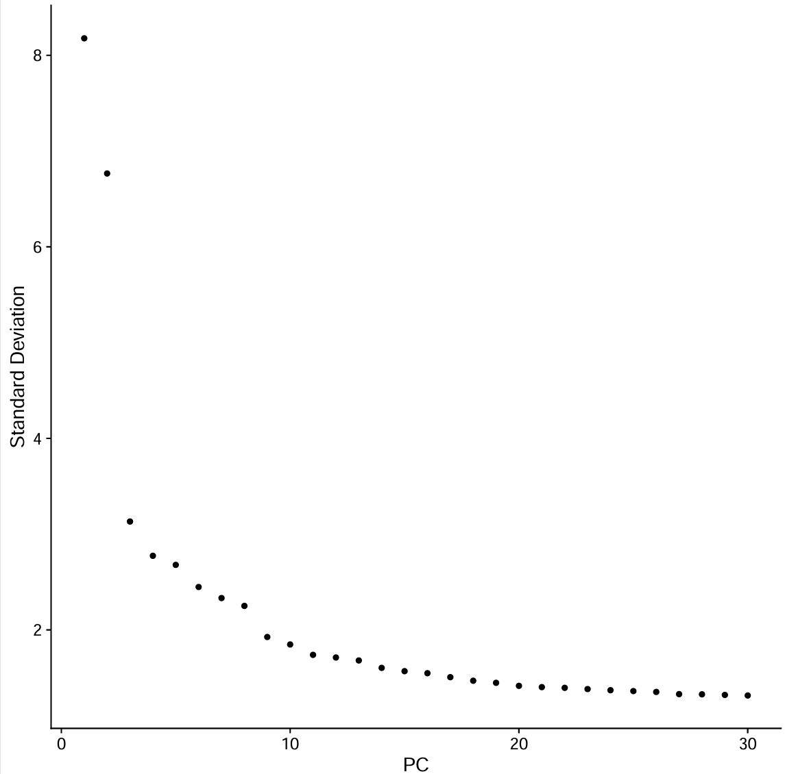
# 选PC数量：ElbowPlot
pdf(file.path(res_dir, "ElbowPlot_all.pdf"))
p <- ElbowPlot(scRNA, ndims = 50, reduction = "pca")
print(p)
dev.off()

跟着教程做复现_GSE157827_7

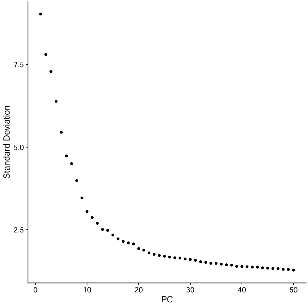
横轴PC序号，纵轴是每个PC解释的方差强度，可以看到：
- 前~10个PC下降很陡
- 到~15-20左右开始明显变平
- 20之后的增益更小
因为教程后面在具体细胞类型用的是pc.num = 1:30，所以这里就也沿用了（教程这里没给用的是多少）。只是更“保守/宽松”，可能把一点噪声也带进邻接图里

如果后面注释发现细胞类型分的过宽泛（很多大类细胞被混成一类），就提高PC/resolution；如果碎成很多小簇、marker不清晰，就降低PC（如1:20）或resolution；如果主要大簇结构和marker注释结论一致，就不用更改

pc.num <- 1:30
# UMAP
scRNA <- RunUMAP(scRNA, dims = pc.num)
# 按AD/NC上色看看整体是否有明显批次/分组分离
p_dim_group <- DimPlot(scRNA, group.by = "group")
# FindNeighbors
scRNA <- FindNeighbors(scRNA, dims = pc.num)
# FindClusters：一次跑多个resolution，方便对比分群“粗/细”
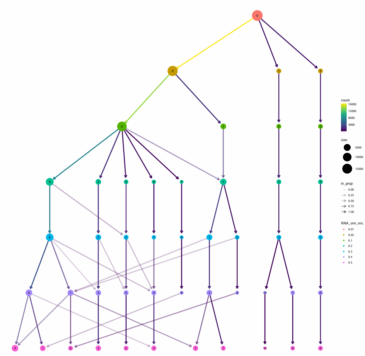
scRNA <- FindClusters(scRNA, resolution = c(0.01, 0.05, 0.1, 0.2, 0.5))
# clustree：看不同resolution之间的聚类“分裂关系”
p_cutree <- clustree(scRNA@meta.data, prefix = "RNA_snn_res.")
# 选一个resolution作为最终cluster标签（教程选0.05）
Idents(scRNA) <- scRNA$RNA_snn_res.0.05
# 把cluster编号标到UMAP上
p_dim_cluster <- DimPlot(scRNA, label = TRUE)
# 拼图展示
pdf(file.path(res_dir, "data_preprocess.pdf"), width = 16, height = 8)
p <- p_dim_group | p_cutree | p_dim_cluster
print(p)
dev.off()

> table(Idents(scRNA))
    0     1    10    11    12     2     3     4     5     6     7     8     9 
44095 41050  2241  1574  1367 19120 13532 12163 11544  9464  7773  2893  2700 

跟着教程做复现_GSE157827_9

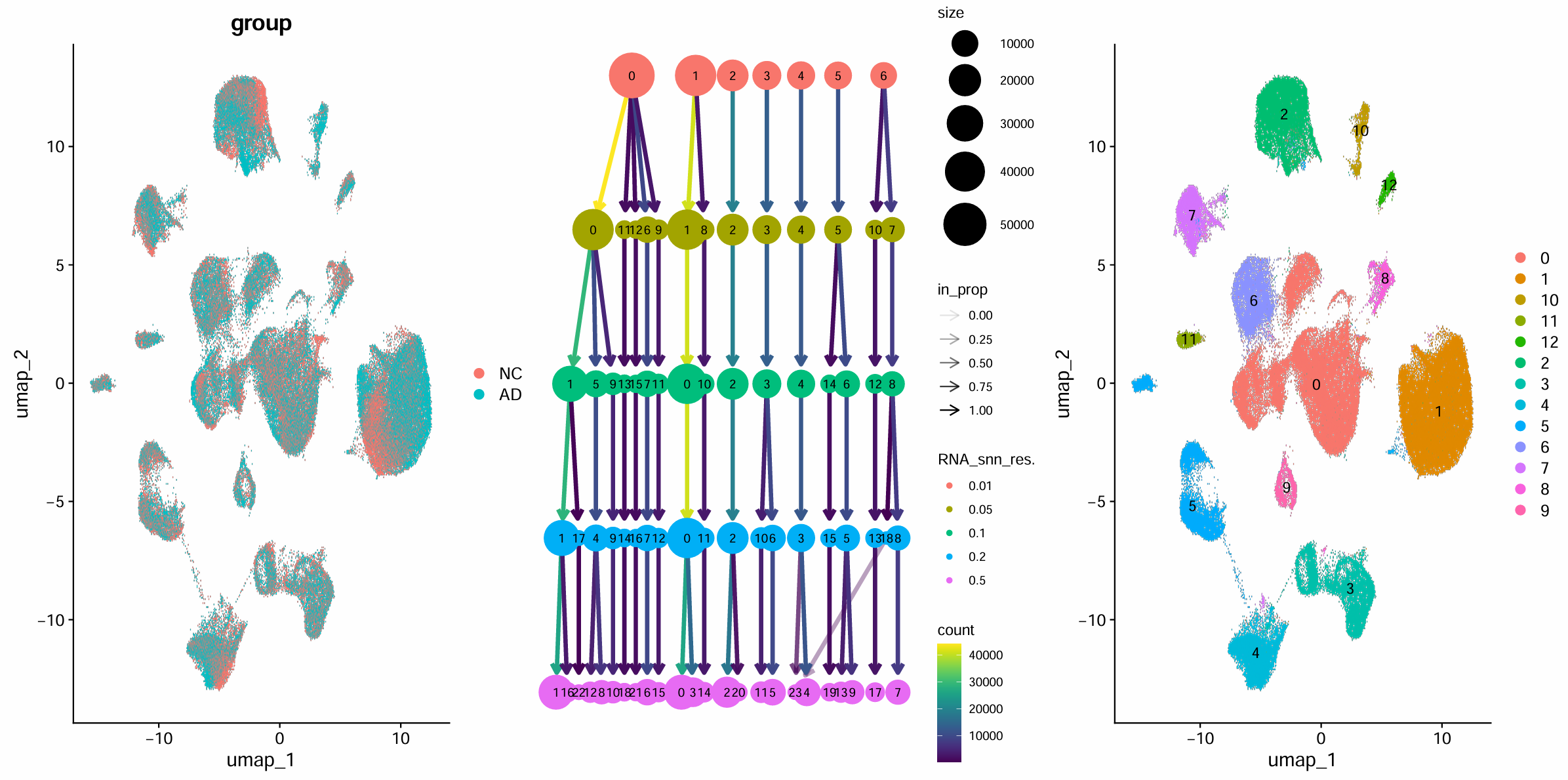
DimPlot：AD/NC是否混在一起

正常情况下，同一细胞类型的AD/NC往往会混在一起（因为细胞类型差异通常比疾病状态更强），如果发现AD和NC几乎完全分成两堆，更常见原因是批次效应/样本差异（例如不同样本测序深度、细胞比例差异等），后面可以再讨论是否要做整合或回归更多变量
clustree：选resolution，resolution越大，cluster越多越细

方法：随着分辨率增大，cluster是不是稳定、是不是“过度碎裂”（出现很多只有几十/几百细胞的小簇）、marker是否清晰（每类marker是否集中在少数几个簇上，如果某个簇同时高表达两类互斥marker，就说明分辨率太低）
- 每一行对应一个分辨率，每个圆点(node)是该分辨率下的一个cluster，圆越大表示细胞越多；连线(edge)表示“上一分辨率的某个簇”在下一分辨率里主要分成了哪些簇；线越粗/越直观代表继承关系越明确、越稳定（基本可理解为“绝大多数细胞都流向同一个子簇”）
- 0.01往往只给你很少的几个大簇，容易把不同细胞类型混在同一簇里，后面做marker注释会比较费劲
- 0.05这一层通常能把数据拆成十来个左右的簇，并且从0.01到0.05的分裂关系比较清楚：大簇分裂成几个仍然比较大的子簇，而不是碎成很多小点。符合“先用一个较粗但能分开大类的分辨率完成主图/主注释”的目标
- 0.1/0.2/0.5更细，但容易“过度分裂”，同一大类细胞会被继续拆成很多子簇，不适合直接做大类注释。可以先用0.05做大类注释，再对某个大类subset后重新聚类，并把resolution提高来做亚群分析
table(Idents(scRNA))：每个cluster大小如果出现极小cluster（比如只有几十个细胞），后面注释时要小心：可能是稀有细胞，也可能是噪声残留

这里发现我使用完整数据的聚类结果竟然有13个簇，反而抽样数据的聚类结果和作者的很类似（只有12个簇），不过似乎UMAP结果不一样是正常的，因为它本身就是随机/近似算法（没设随机种子时，形状、旋转、间距都会变），这些差异通常只影响“图长什么样”，不一定影响生物学结论，但后面细胞类型注释时就需要自己分析一下，不能直接照抄作者的对应关系

细胞类型注释

library(Seurat)
library(tidyverse)
library(patchwork)

看marker基因在各聚类中的表达情况

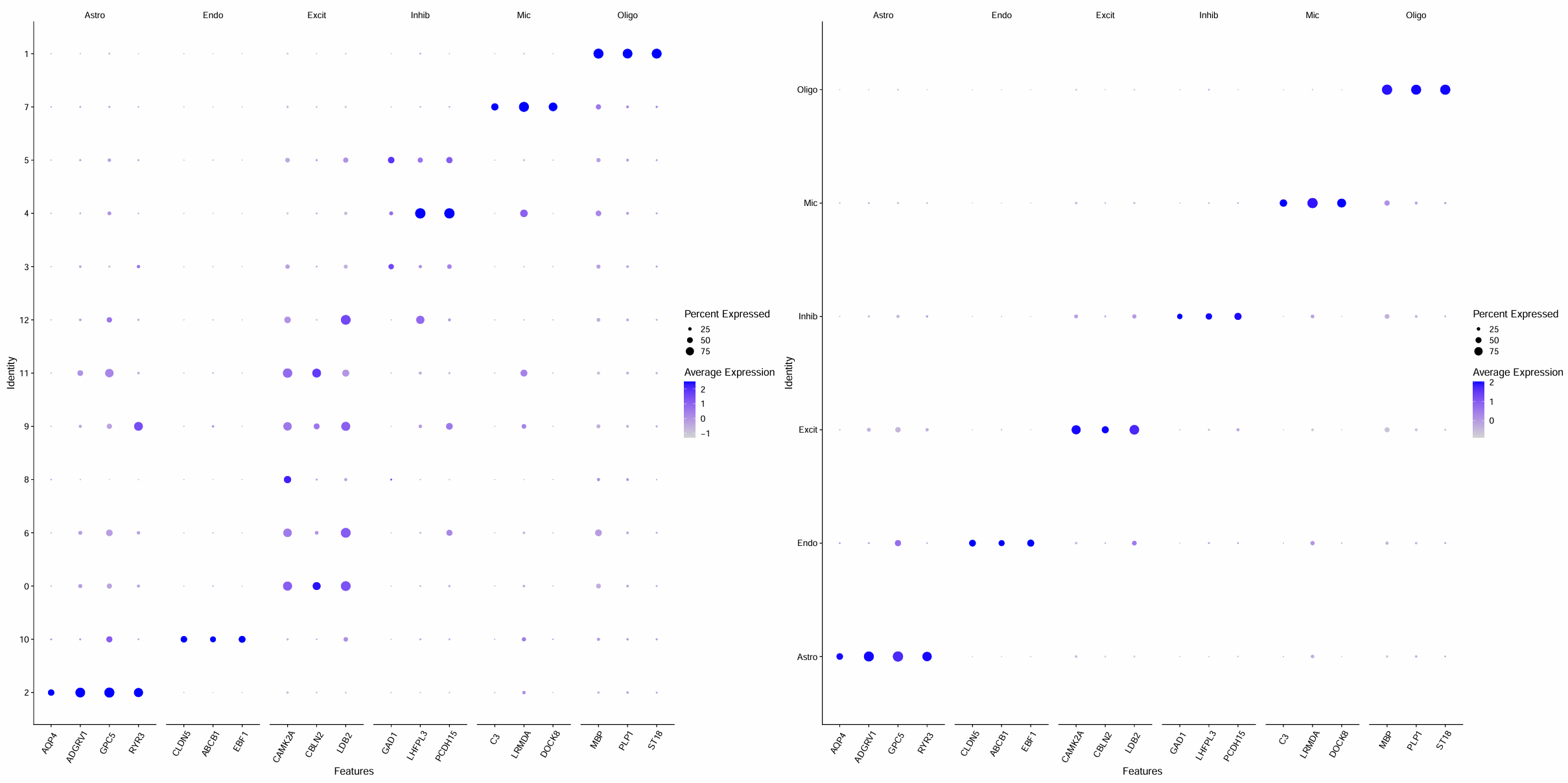
# 每个细胞的marker基因
astrocytes  <- c("AQP4", "ADGRV1", "GPC5", "RYR3")
endothelial <- c("CLDN5", "ABCB1", "EBF1")
excitatory  <- c("CAMK2A", "CBLN2", "LDB2")
inhibitory  <- c("GAD1", "LHFPL3", "PCDH15")
microglia   <- c("C3", "LRMDA", "DOCK8")
oligodendro <- c("MBP", "PLP1", "ST18")
# 画图展示各个聚类中marker基因的表达量
p_astro <- DotPlot(scRNA, features = astrocytes)  + RotatedAxis() + ggtitle("Astro markers")
p_endo  <- DotPlot(scRNA, features = endothelial) + RotatedAxis() + ggtitle("Endo markers")
p_exc   <- DotPlot(scRNA, features = excitatory)  + RotatedAxis() + ggtitle("Excit markers")
p_inh   <- DotPlot(scRNA, features = inhibitory)  + RotatedAxis() + ggtitle("Inhib markers")
p_mic   <- DotPlot(scRNA, features = microglia)   + RotatedAxis() + ggtitle("Micro markers")
p_oligo <- DotPlot(scRNA, features = oligodendro) + RotatedAxis() + ggtitle("Oligo markers")
# 拼图展示
pdf(file.path(res_dir, "cluster_marker_gene.pdf"), width = 10, height = 15)
p <- (p_astro | p_endo) / (p_exc | p_inh) / (p_mic | p_oligo)
print(p)
dev.off()

抽样数据：

跟着教程做复现_GSE157827_10

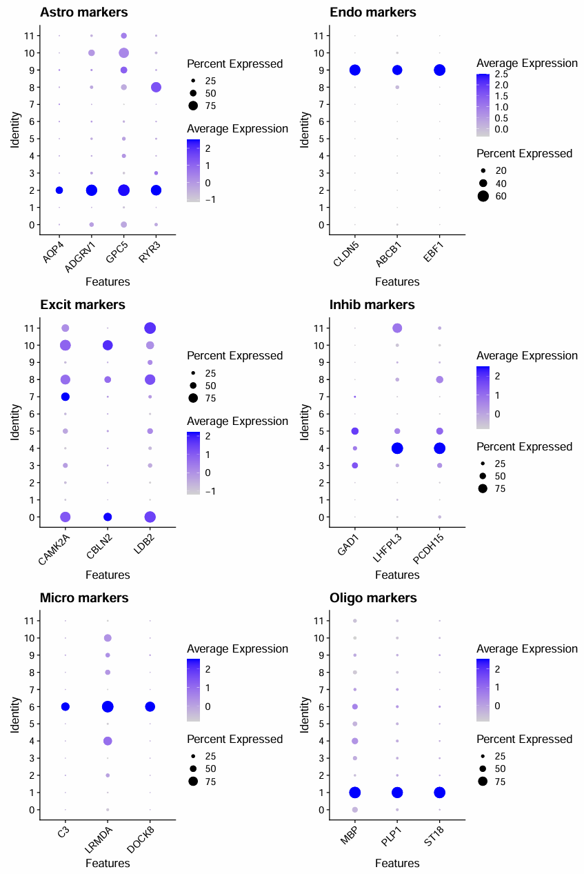
Oligodendrocyte：1
Astrocyte：2
Microglia：6
Endothelial：9
Inhibitory neuron：4
Excitatory neuron：7、0、10、11、8
- 因为7的CAMK2A表达很强，就把它划进Excit里面（教程作者也是这么做的，我的7对应他的9，都是CAMK2A表达高而另外两个没啥表达的情况）
不确定：5、3

全部数据：

跟着教程做复现_GSE157827_11

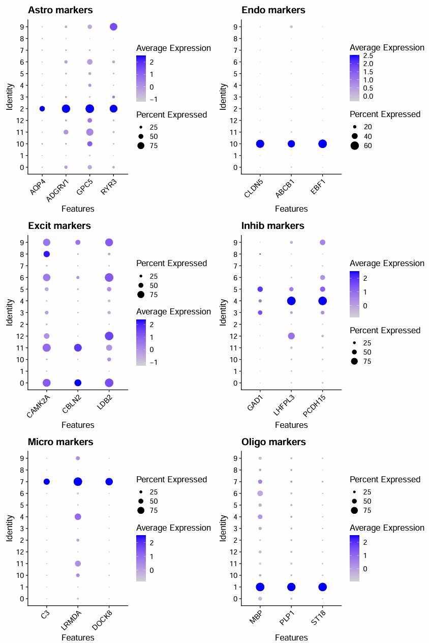
Oligodendrocyte：1
Astrocyte：2
Microglia：7
Endothelial：10
Inhibitory neuron：4
Excitatory neuron：8、0、11、6、9、12
不确定：5、3

又画了第二组图来辅助判断

check_markers <- list(
  Neuron   = c("RBFOX3","SNAP25"),
  Excit    = c("SLC17A7","SATB2"),
  Inhib    = c("GAD2","SLC6A1"),
  OPC      = c("PDGFRA","CSPG4"),
  Pericyte = c("RGS5","PDGFRB"),
  Micro2   = c("P2RY12","CX3CR1","AIF1"),
  Astro2   = c("ALDH1L1","SLC1A2","GFAP"),
  Oligo2   = c("MOG","MAG","OLIG1","OLIG2"),
  Endo2    = c("KDR","PECAM1","VWF")
)
pdf(file.path(res_dir, "cluster_marker_gene2.pdf"), width = 20, height = 20)
p <- DotPlot(scRNA, features = unlist(check_markers)) + RotatedAxis()
print(p)
dev.off()

抽样数据：

跟着教程做复现_GSE157827_12

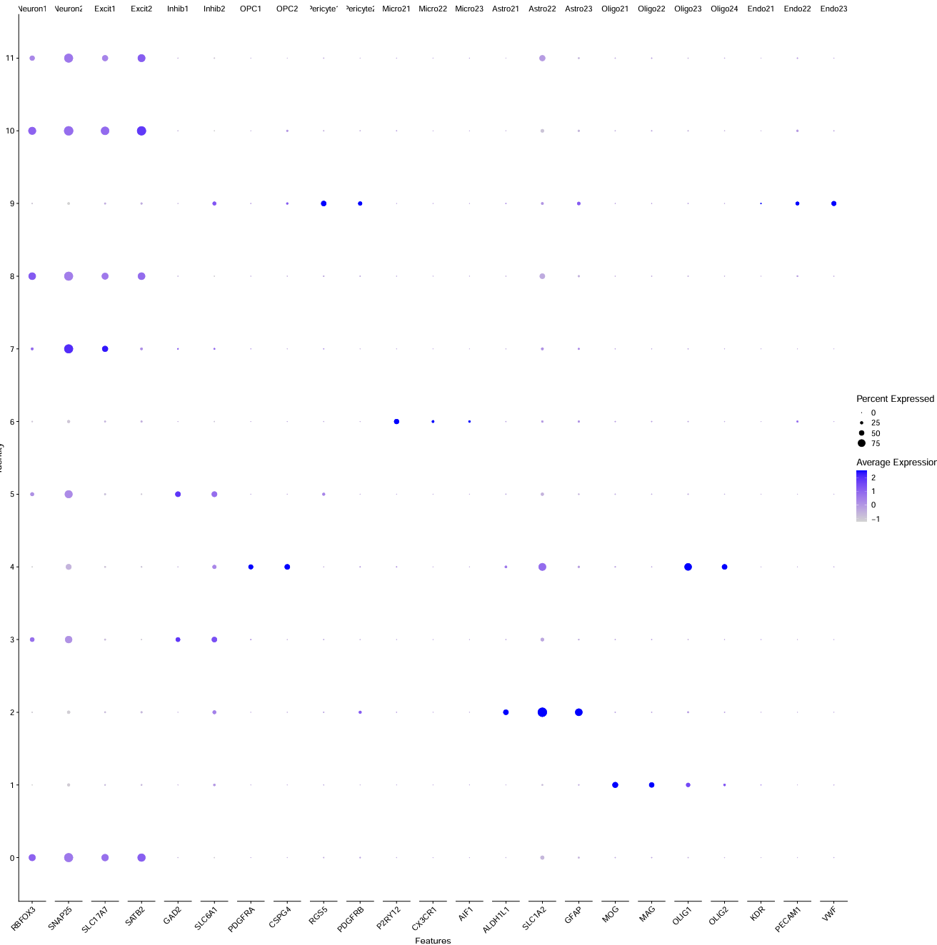
全部数据：

跟着教程做复现_GSE157827_13

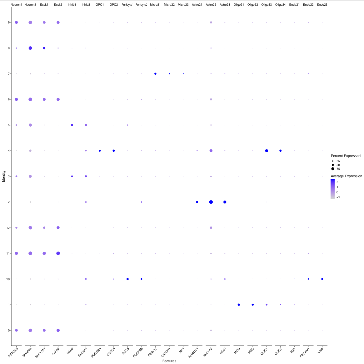
最后还是把5、3都认定成Inhibitory neuron了

改细胞类型

cluster2type <- c(
  "0"  = "Excit",
  "1"  = "Oligo",
  "2"  = "Astro",
  "3"  = "Inhib",
  "4"  = "Inhib",
  "5"  = "Inhib",
  "6"  = "Mic",
  "7"  = "Excit",
  "8"  = "Excit",
  "9"  = "Endo",
  "10" = "Excit",
  "11" = "Excit"
)
# cluster2type <- c(
#   "0"  = "Excit",
#   "1"  = "Oligo",
#   "2"  = "Astro",
#   "3"  = "Inhib",
#   "4"  = "Inhib",
#   "5"  = "Inhib",
#   "6"  = "Excit",
#   "7"  = "Mic",
#   "8"  = "Excit",
#   "9"  = "Excit",
#   "10" = "Endo",
#   "11" = "Excit",
#   "12" = "Excit"
# )
scRNA$celltype <- unname(cluster2type[as.character(Idents(scRNA))])

> # 检测一下有没有NA（有没有cluster没被映射到）
> table(scRNA$celltype, useNA = "ifany")
Astro  Endo Excit Inhib   Mic Oligo 
19120  2241 62093 37239  7773 41050 

画图展示最终注释结果

gene_list <- list(
  Astro = astrocytes,
  Endo = endothelial,
  Excit = excitatory,
  Inhib = inhibitory,
  Mic = microglia,
  Oligo = oligodendro
)
scRNA@active.ident <- factor(scRNA@active.ident, levels = c(2, 9, 0, 7, 8, 10, 11, 3, 4, 5, 6, 1))
# scRNA@active.ident <- factor(scRNA@active.ident, levels = c(2, 10, 0, 6, 8, 9, 11, 12, 3, 4, 5, 7, 1))
p_dot_1 <- DotPlot(scRNA, features = gene_list, assay = "RNA") +
  theme(axis.text.x = element_text(angle = 60, vjust = 0.8, hjust=0.8))
Idents(scRNA) <- scRNA$celltype
scRNA@active.ident <- factor(scRNA@active.ident, levels = c("Astro", "Endo", "Excit", "Inhib", "Mic", "Oligo"))
p_dot_2 <- DotPlot(scRNA, features = gene_list, assay = "RNA") +
  theme(axis.text.x = element_text(angle = 60, vjust = 0.8, hjust=0.8))
# 每个聚类/注释后大类的marker基因表达量情况
pdf(file.path(res_dir, "cluster_marker_gene_final.pdf"), width = 30, height = 15)
p <- p_dot_1 | p_dot_2
print(p)
dev.off()
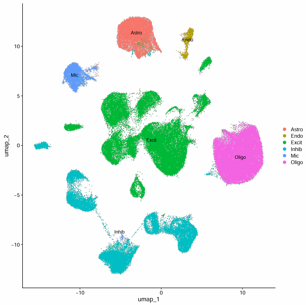
# UMAP图标注细胞类型后
pdf(file.path(res_dir, "cluster_marker_gene_result.pdf"), width = 10, height = 10)
p <- DimPlot(scRNA, label = T)
print(p)
dev.off()
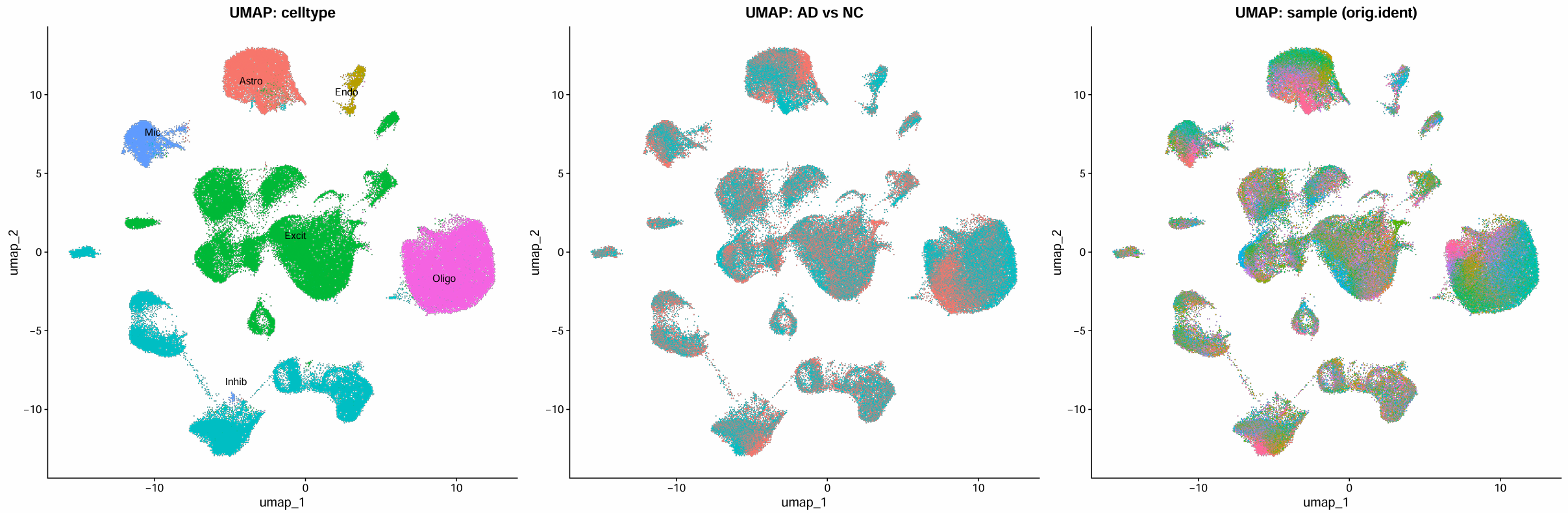
# 总结：UMAP图分别按细胞类型/诊断信息/样本分组
p_type <- DimPlot(scRNA, group.by = "celltype", label = TRUE, repel = TRUE) +
  NoLegend() +
  ggtitle("UMAP: celltype")
p_grp <- DimPlot(scRNA, group.by = "group") +
  NoLegend() +
  ggtitle("UMAP: AD vs NC")
p_samp <- DimPlot(scRNA, group.by = "orig.ident", raster = TRUE) +
  NoLegend() +
  ggtitle("UMAP: sample (orig.ident)")
pdf(file.path(res_dir, "cluster_marker_gene_summary.pdf"), width = 24, height = 8)
p <- p_type | p_grp | p_samp
print(p)
dev.off()
# 保存结果
saveRDS(
    scRNA, 
    file = file.path("C:\\Users\\17185\\Desktop\\hERV_calc\\GSE157827\\data", "GSE157827_celltype.rds"), 
    compress = "xz"
)

跟着教程做复现_GSE157827_14

跟着教程做复现_GSE157827_15

跟着教程做复现_GSE157827_16

复现论文中的图片

跟着教程做复现_GSE157827_16_1

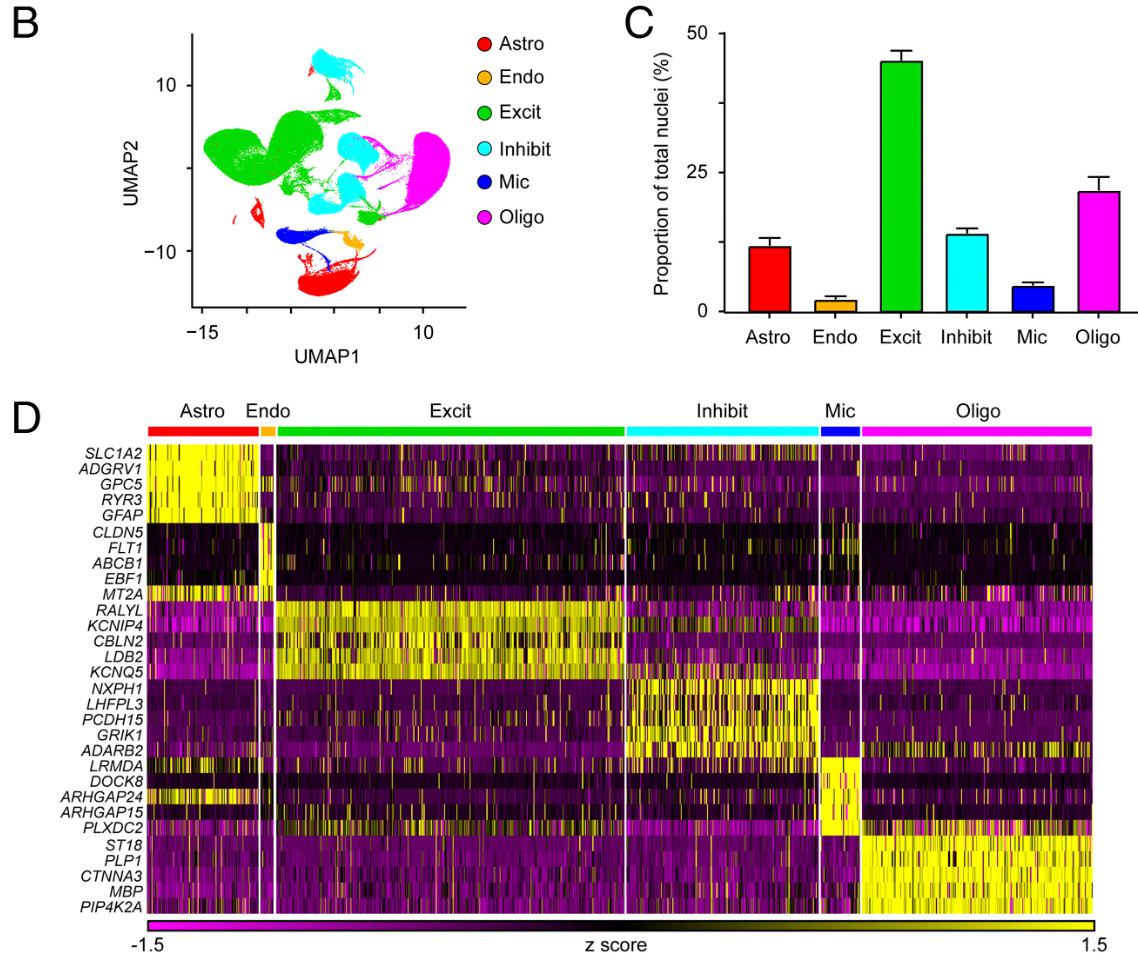
# Fig 1B：UMAP按细胞类型上色
ct_cols <- c(
  Astro = "#1b9e77",
  Endo  = "#d95f02",
  Excit = "#7570b3",
  Inhib = "#e7298a",
  Mic   = "#66a61e",
  Oligo = "#e6ab02"
)
fig_1b <- DimPlot(
  scRNA, 
  reduction = "umap", 
  cols = ct_cols, 
  label = FALSE
)

# Fig 1C：统计各细胞类型的细胞数和比例
ct_stat <- as.data.frame(table(scRNA$celltype))
colnames(ct_stat) <- c("celltype", "total")
ct_stat$celltype <- factor(ct_stat$celltype, levels = levels(scRNA@active.ident))
ct_stat$percentage <- 100 * ct_stat$total / sum(ct_stat$total)
fig_1c <- ggplot(ct_stat, aes(x = celltype, y = percentage, fill = celltype)) +
  geom_bar(stat = "identity", color = "black") +
  scale_fill_manual(values = ct_cols) +
  theme_classic() +
  theme(axis.title.x = element_blank(), legend.position = "none") +
  ylab("Proportion of total nuclei (%)")

# Fig 1D：各细胞类型top marker热图

# 抽取细胞（节省时间）
set.seed(1)
CTs <- levels(scRNA@active.ident)  # 用 levels 保持顺序
sampled <- unlist(lapply(CTs, function(ct){
  cells <- WhichCells(scRNA, idents = ct)
  if (length(cells) > 3000) sample(cells, 3000) else cells
}))
scRNA <- scRNA[, sampled]
# 因为想尽可能准确，最后画结果图时就没有抽取细胞

# 第一种方法：直接找每个细胞类型的marker
diff.wilcox1 <- FindAllMarkers(scRNA, test.use = "wilcox", only.pos = TRUE)
all_markers1 <- diff.wilcox1 %>%  # 过滤：p_val<0.05 且logFC>0.5
  select(gene, everything()) %>%
  subset(p_val<0.05 & abs(diff.wilcox1$avg_log2FC) > 0.5)
top51 <- all_markers1 %>%  # 根据avg_log2FC取每类top5 marker
  group_by(cluster) %>%
  top_n(n = 5, wt = avg_log2FC)
top51 <- CaseMatch(search = as.vector(top51$gene), match = rownames(scRNA))
scRNA <- ScaleData(scRNA, features = top51)
fig_1d_1 <- DoHeatmap(
  scRNA,
  features = top51,
  angle = 0,
  group.colors = unname(ct_cols),
  disp.min = -2.5,
  disp.max = 2.5
)
# 拼图展示
pdf(file.path(res_dir, "paper1B-D.pdf"), width = 24, height = 16)
p <- (fig_1b + labs(tag = "B")) + (fig_1c + labs(tag = "C")) / (fig_1d_1 + labs(tag = "D"))
print(p)
dev.off()

跟着教程做复现_GSE157827_17

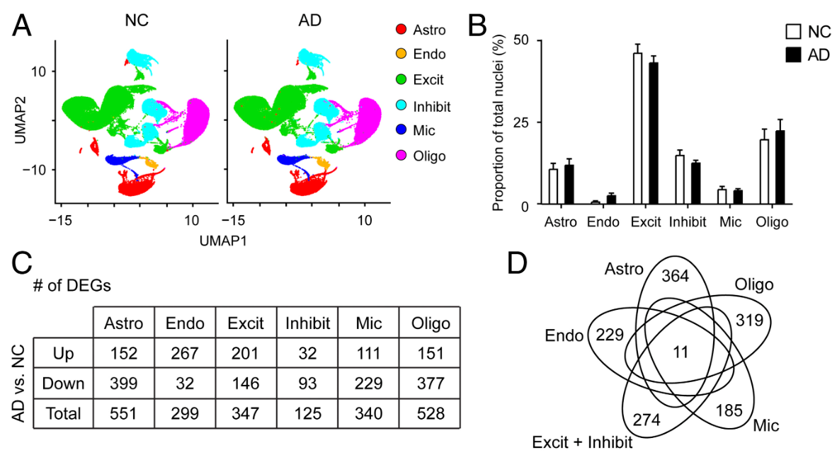
Fig 1B：UMAP按细胞类型上色。主要看
- 同一类型是否聚成相对连续的区域（说明注释/聚类一致性不错）
- 不同类型之间的相对位置：脑组织里常见现象是神经元（Excit/Inhib）形成大块区域，胶质细胞（Oligo/Astro/Mic）分在不同“岛”上，内皮（Endo）通常是一小块独立岛
Fig 1C：统计各细胞类型的细胞数和比例
- 通常Excit会最多，其次可能是Oligo/Inhib
- 如果某一类异常少（比如Endo或Mic极少）并不一定错，可能是由于组织本身含量低、或QC/过滤阈值导致这一类更容易被过滤
Fig 1D：各细胞类型top marker热图。每个细胞类型做FindAllMarkers，根据logFC选top5 marker，然后DoHeatmap。应该看到每个细胞类型都有一组“只在自己那一块变深”的marker
- Astro：AQP4/SLC1A2/ALDH1L1…
- Endo：CLDN5/PECAM1/VWF…
- Oligo：MBP/PLP1/MOG…
- Mic：C3/AIF1/P2RY12…
- Excit：SLC17A7/SATB2…
- Inhib：GAD1/2/SLC6A1…

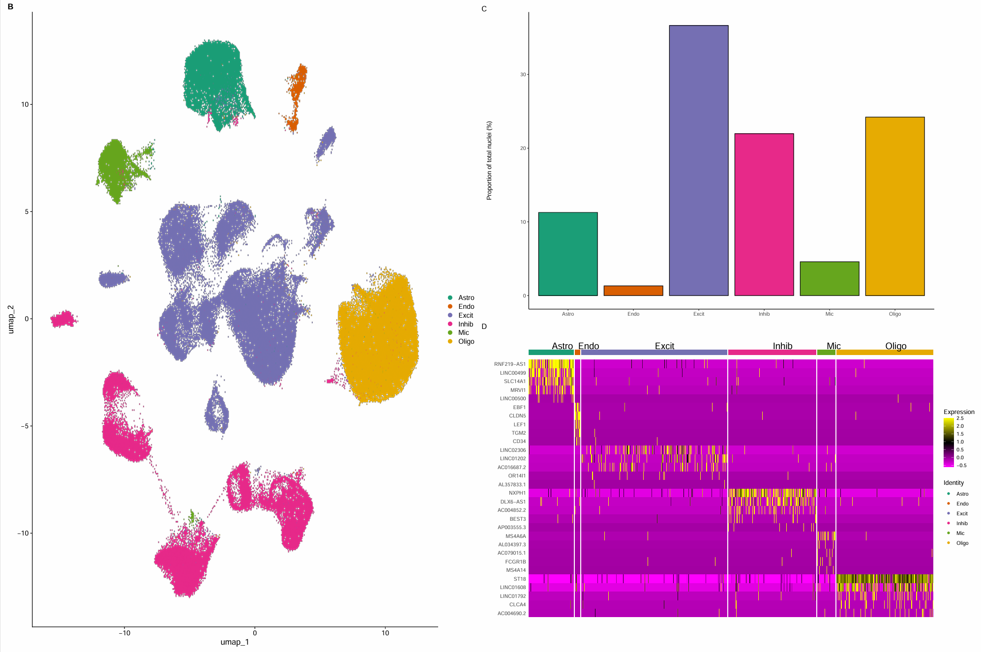
发现我的热图好像跟作者的不太一样，于是选择只在高变基因里FindAllMarkers，并并剔除明显的lncRNA/未知转录本

# 第二种方法：只在高变基因里找marker，并剔除明显的lncRNA/未知转录本
diff.wilcox2 <- FindAllMarkers(
  scRNA,
  only.pos = TRUE,
  features = VariableFeatures(scRNA)
)
all_markers2 <- diff.wilcox2 %>%
  select(gene, everything()) %>%
  subset(p_val<0.05 & abs(diff.wilcox2$avg_log2FC) > 0.5) %>%
  filter(!grepl("^LINC", gene),
         !grepl("^AC", gene),
         !grepl("^AL", gene),
         !grepl("^AP", gene))
top52 <- all_markers2 %>%
  group_by(cluster) %>%
  top_n(n = 5, wt = avg_log2FC)
top52 <- CaseMatch(search = as.vector(top52$gene), match = rownames(scRNA))
scRNA <- ScaleData(scRNA, features = top52)
fig_1d_2 <- DoHeatmap(
  scRNA,
  features = top52,
  angle = 0,
  group.colors = unname(ct_cols),
  disp.min = -2,
  disp.max = 2
)
pdf(file.path(res_dir, "paper1D_2.pdf"), width = 15, height = 10)
print(fig_1d_2)
dev.off()

跟着教程做复现_GSE157827_18

这回基因名差不多了，但似乎颜色还有点差别。因此直接到原文中看了下作者的图，似乎基因选的都是经典marker（虽然论文中标的是top5差异）

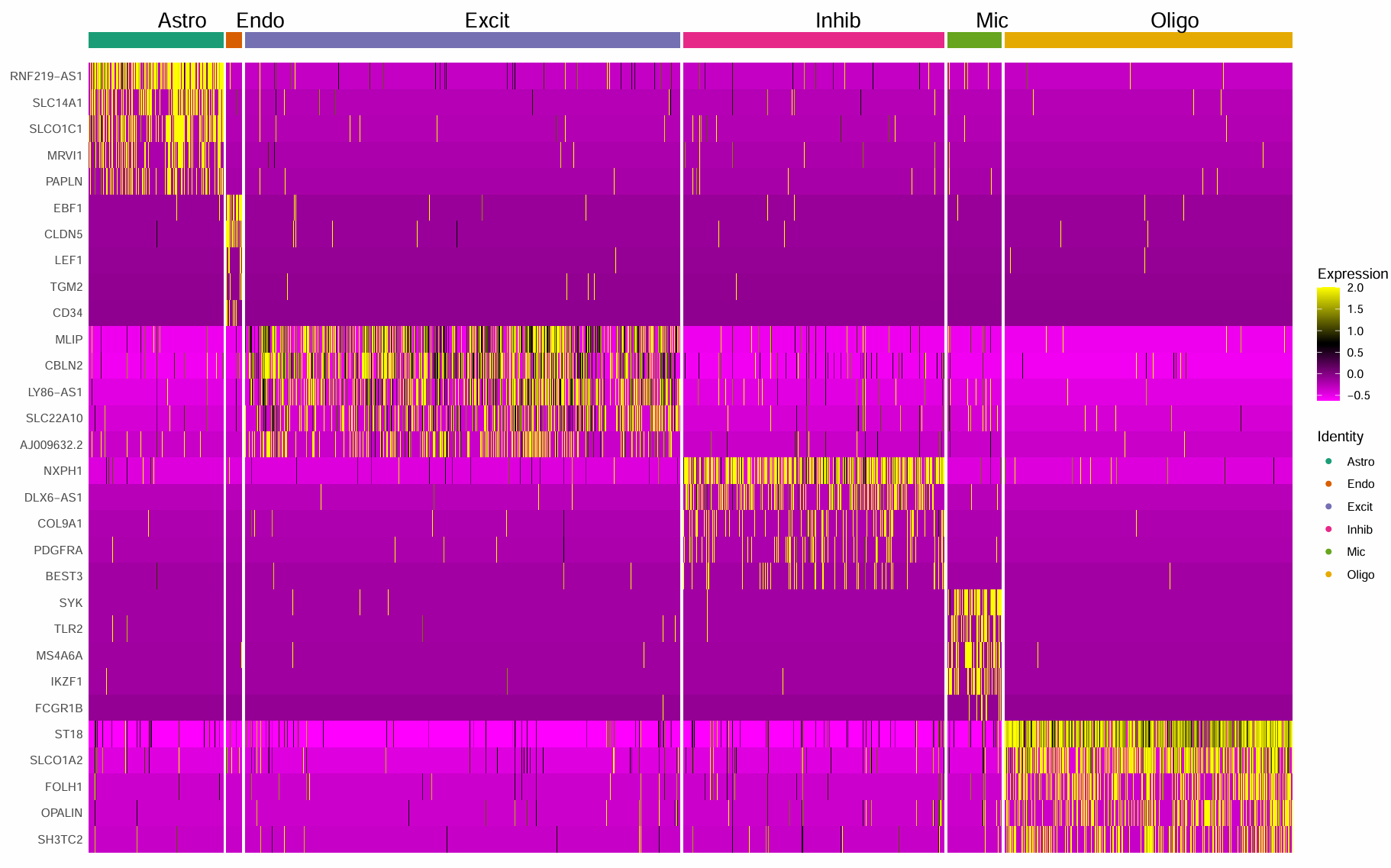
# 第三种方法：直接指定marker（根据作者论文的图）
genes_paper <- c(
  "SLC1A2","ADGRV1","GPC5","RYR3","GFAP",
  "CLDN5","FLT1","ABCB1","EBF1","MT2A",
  "RALYL","KCNIP4","CBLN2","LDB2","KCNQ5",
  "NXPH1","LHFPL3","PCDH15","GRIK1","ADARB2",
  "LRMDA","DOCK8","ARHGAP24","ARHGAP15","PLXDC2",
  "ST18","PLP1","CTNNA3","MBP","PIP4K2A"
)
genes_use <- intersect(genes_paper, rownames(scRNA))
length(genes_use) == length(genes_paper)  # 全在我的数据集中
scRNA <- ScaleData(scRNA, features = genes_use, verbose = FALSE)
p <- DoHeatmap(
  scRNA,
  features = genes_use,
  disp.min = -1.5,
  disp.max = 1.5,
  angle = 0,
  group.colors = unname(ct_cols)
) + scale_fill_gradientn(
  colors = c("#f100ef", "black", "#f0e442"),
  limits = c(-1.5, 1.5)
)
pdf(file.path(res_dir, "paper1D_3.pdf"), width = 15, height = 10)
print(p)
dev.off()

跟着教程做复现_GSE157827_19

这回就差不多了，大概还是用的基因不太一样，导致scale后的数据值不太一样，于是DoHeatmap的颜色我的就偏粉、作者的就偏黑

我在论文原文中看到这个图的描述是“Heatmap showing the top five most enriched genes for each cell type”，然后作者还列出了各基因的p值和logFC，说明似乎作者并不是用指定marker的方式来画的图，而且也没有过滤LINC/AP/AL/AC。如果作者也是用FindAllMarkers这类方法做的，那么可能是什么因素导致我和作者的结果不一样（除了版本/抽取部分数据/随机数seed的因素）

原文在FindClusters时用来更高的分辨率，然后在更多的clusters中FindAllMarkers，而我的是先合并成6个细胞类型，再在每个clusters中FindAllMarkers，这样得到的top5可能不一致（celltype-level更粗，容易被“细胞类型内部异质性”稀释）
原文的p值阈值为0.1，而我用的是0.05，并且我还设置了logFC的阈值，容易筛出“表达很稀疏、但在某一类细胞里偶尔高表达的转录本”
上游处理不一致，原文做了21个样本的整合等处理，教程中没有作整合，直接merge合并（这步在自己拿STAR原始计数数据做时要注意，是不是也要先按原文的方法做整合）

基于细胞类型的AD/NC差异分析

library(Seurat)
library(tidyverse)
library(patchwork)
library(gridExtra)
library(VennDiagram)
library(ggplotify)
library(grid)
scRNA <- readRDS("C:\\Users\\17185\\Desktop\\hERV_calc\\GSE157827\\data\\GSE157827_celltype.rds")
DefaultAssay(scRNA) <- "RNA"
scRNA$group <- factor(scRNA$group, levels = c("NC","AD"))
scRNA$celltype <- factor(
  scRNA$celltype,
  levels = c("Astro","Endo","Excit","Inhib","Mic","Oligo")
)
Idents(scRNA) <- scRNA$celltype

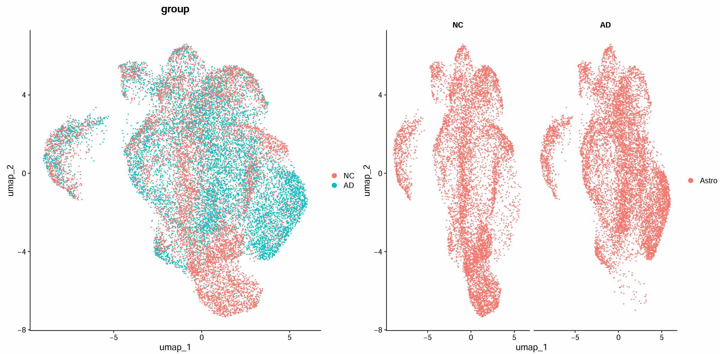
先看AD/NC两组在UMAP上的细胞类型分布是否一致
比较两组中各细胞类型的组成比例
在每个细胞类型内部做AD-NC的差异表达
把各细胞类型的差异基因集合做交集/特异性展示

跟着教程做复现_GSE157827_20

统计细胞类型在AD/NC中的分布和比例

# fig_2a
ct_cols <- c('#1b9e77','#d95f02','#7570b3','#e7298a','#66a61e','#e6ab02')
fig_2a <- DimPlot(scRNA, split.by = "group", cols = ct_cols)
# fig_2b
ct_stat2 <- as.data.frame(table(scRNA$celltype, scRNA$group))
colnames(ct_stat2) <- c("celltype","group","n")
ct_stat2 <- ct_stat2 %>%
  group_by(group) %>%
  mutate(percentage = n / sum(n)) %>%
  ungroup()
ct_stat2$group <- factor(ct_stat2$group, levels = c("NC","AD"))
ct_stat2$celltype <- factor(ct_stat2$celltype, levels = levels(scRNA$celltype))
fig_2b <- ggplot(
  ct_stat2, 
  aes(x = celltype, fill = group, y = percentage)
) +
  geom_bar(
    position = position_dodge(width = 0.8), 
    width = 0.6,
    stat = "identity", 
    color = "black"
  ) +
  scale_fill_manual(values = c('white','black')) +
  theme_classic() +
  ylab("Proportion of total nuclei (%)") +
  theme(
    axis.title.x = element_blank(),
    legend.title = element_blank()
  )

每个细胞类型中做AD-NC差异表达

“只在同一种细胞类型内部”比较AD-NC：避免把“细胞类型差异”误当成“疾病差异”

# 在每个细胞类型内平衡AD/NC细胞数：避免同一个细胞类型内，AD或NC的细胞数显著大于另一边
balance_cells <- function(obj, ct){
  sub <- subset(obj, idents = ct)
  ad <- WhichCells(sub, expression = group == "AD")
  nc <- WhichCells(sub, expression = group == "NC")
  if(length(ad) > 2000){
    n <- min(length(ad), length(nc))
    sub[, c(sample(ad, n), sample(nc, n))]
  } else {
    sub
  }
}
cts <- levels(scRNA$celltype)
obj_bal <- merge(x = balance_cells(scRNA, cts[1]),
                 y = lapply(cts[-1], \(ct) balance_cells(scRNA, ct)))
obj_bal$celltype <- factor(
  obj_bal$celltype,
  levels = c("Astro","Endo","Excit","Inhib","Mic","Oligo")
)
obj_bal <- JoinLayers(obj_bal, assay = "RNA")
# 构造分组（AD/NC-细胞类型）
obj_bal$compare <- paste(obj_bal$group, obj_bal$celltype, sep = "_")
scRNA$compare <- paste(scRNA$group, scRNA$celltype, sep = "_")
table(scRNA$compare)
table(obj_bal$compare)
# 每个细胞类型运行一次FindMarkers
ct <- levels(obj_bal$celltype)
all_markers <- lapply(ct, function(x){
  message("Running: ", x)
  FindMarkers(
    obj_bal,
    group.by = "compare",
    ident.1 = paste0("AD_", x),
    ident.2 = paste0("NC_", x),
    logfc.threshold = 0.25,
    min.pct = 0.1
  )
})
names(all_markers) <- ct
lapply(all_markers, nrow)
# 筛显著DEG，并汇总每类Up/Down数量
all_markers_sig <- lapply(all_markers, function(df){
  df2 <- subset(  # p值<0.1
    df, 
    p_val_adj < 0.1
  )
  return(df2)
})
# 保存结果
save(all_markers_sig, file = "C:\\Users\\17185\\Desktop\\hERV_calc\\GSE157827\\data\\GSE157827_all_markers_sig.RData")
# 统计每个细胞类型Up/Down/Total
marker_stat <- sapply(all_markers_sig, function(df){
  c(
    Up    = sum(df$avg_log2FC > 0),
    Down  = sum(df$avg_log2FC < 0),
    Total = nrow(df)
  )
})
marker_stat <- as.data.frame(marker_stat)
# fig_2c 
fig_2c <- ggpubr::as_ggplot(
  tableGrob(marker_stat, theme = ttheme_default(base_size = 25))
)
# fig_2d
Astro <- rownames(all_markers_sig$Astro)
Endo  <- rownames(all_markers_sig$Endo)
Mic   <- rownames(all_markers_sig$Mic)
Oligo <- rownames(all_markers_sig$Oligo)
`Excit+Inhib` <- unique(
  c(rownames(all_markers_sig$Excit),
  rownames(all_markers_sig$Inhib))
)
veen_eles2 <- list(
  Astro = Astro,
  Endo = Endo,
  `Excit+Inhib` = `Excit+Inhib`,
  Mic = Mic,
  Oligo = Oligo
)
plt <- venn.diagram(veen_eles2, filename = NULL)
fig_2d <- as.ggplot(function() grid.draw(grobTree(plt)))
pdf(file.path(res_dir, "paper2A-D.pdf"), width = 30, height = 18)
p <- (fig_2a + fig_2b) / (fig_2c + fig_2d) + plot_annotation(tag_levels = "A")
print(p)
dev.off()

跟着教程做复现_GSE157827_21

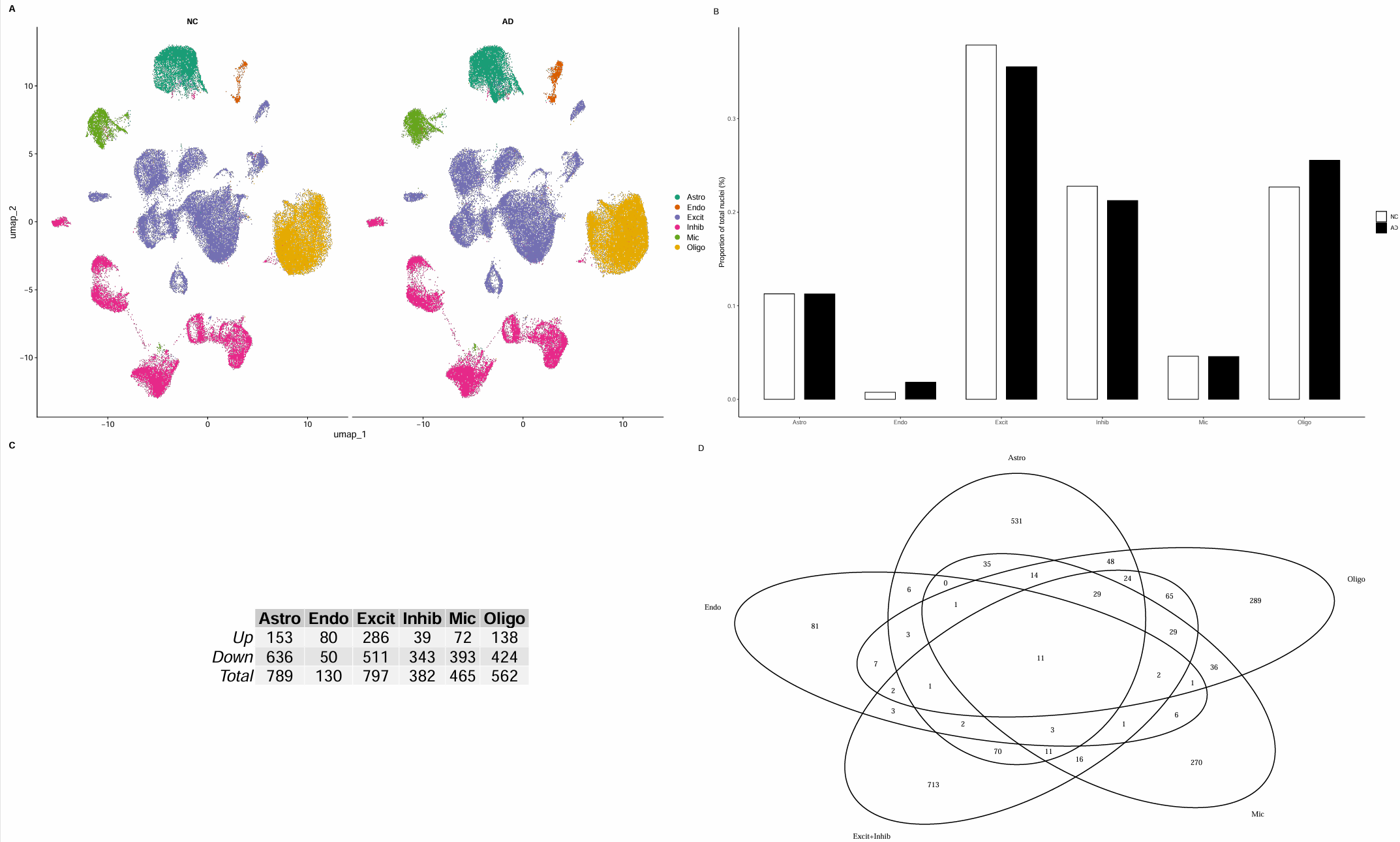
Fig 2A：按组拆分的UMAP。同一种细胞类型（同颜色）在两组里是否出现在相似位置、形状是否相近
Fig 2B：两组中各细胞类型的比例。这是“细胞组成差异”，不等同于“基因表达差异”，能提示后面哪些细胞类型的生物学变化更值得关注
Fig 2C：按论文阈值筛显著DEG，并汇总每类Up/Down数量。每列一个细胞类型，Up/Down/Total反映在该细胞类型中，AD相比NC有多少显著上调/下调基因
- “Total值特别大”的细胞类型，部分原因可能是因为其细胞数更多，所以它更多是“变化规模提示”，而不是严格可比的效应量
Fig2D：不同细胞类型的DEG交集。取各细胞类型的显著DEG基因名集合，然后做Venn，并把Excit和Inhib合并成一个集合
- 每个圈：该细胞类型的显著DEG集合
- 交集：多个细胞类型共同变化的基因
- “只在某个圈里”的部分：该细胞类型特异的变化（通常更接近机制/细胞功能变化）

在第一次按教程代码找的时候，我和作者找的差异基因数量级差了很多：

直接对每个细胞类型来FindMarkers，只要求logFC和p值0.1，当有几万细胞时，，哪怕非常小的差异也会变成极小p值，导致total的数量很多
之前细胞类型注释时不够细分，把一些其他小的细胞类型混了进去，让Inhib和Endo变成了“混合类”，AD/NC在这些“混合类”里的亚群比例不同，产生大量“伪差异”，尤其造成Down的数量极多（因为两组里细胞组成/质量差异会体现为广泛下调）

跟着教程做复现_GSE157827_22

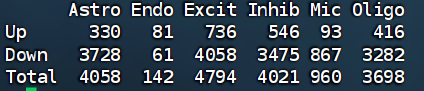
可能的解决方法：

提高阈值：|logFC|>0.25 min.pct=0.1或0.2
平衡AD/NC的细胞数（让每个细胞类型中AD和NC的细胞数相同）
用MAST加入协变量
按donor/sample做pseudo-bulk再DE

我这里采用平衡细胞数和提高阈值的方法

跟着教程做复现_GSE157827_23

pseudo-bulk：把单细胞/单核数据按“样本×细胞类型”汇总成“伪bulk表达矩阵”，再按样本作为重复做差异分析

以这个数据为例，我现在有21个样本，对每个细胞类型分别做：
在每个样本内，把该细胞来信的原始counts按基因求和，得到一个“bulk-like”的矩阵（gene × sample）
之后向传统RNA-seq一样用edgeR/DESeq2等方法做差异表达分析

和论文里“按细胞做DE”的方法相比：

统计单位变成“样本/个体”而不是“细胞”，避免把同一个人的几千个细胞当成几千个独立重复，因此DEG通常更“保守”、可重复性更好
“按细胞做DE”实现简单、速度快，细胞数大时“很容易显著”，能挖到很多差异基因，但因为“同一donor的细胞彼此相关，但统计检验当它们独立”，所以p值偏小，DEG数量可能虚高。同时很难正确加入donor-level协变量（age/sex/PMD）并解释“组间差异”是否只是样本构成差异

一个简单的示例：

library(edgeR)
# 按celltype+orig.ident汇总原始counts
pb_list <- AggregateExpression(
  scRNA,
  assays = "RNA",
  group.by = c("celltype", "orig.ident"),
  slot = "counts",
  return.seurat = FALSE
)
pb_counts <- pb_list$RNA
# 构造样本级meta（每个orig.ident一行）
sample_meta <- scRNA@meta.data |>
  dplyr::distinct(orig.ident, group, .keep_all = FALSE)
sample_meta$orig.ident <- as.character(sample_meta$orig.ident)
sample_meta$group <- factor(sample_meta$group, levels = c("NC","AD"))
pb_meta <- data.frame(pb_id = colnames(pb_counts))
pb_meta$orig.ident <- str_extract(pb_meta$pb_id, "[^_]+$")
pb_meta$celltype   <- str_replace(pb_meta$pb_id, "_[^_]+$", "")
pb_meta$group <- sample_meta$group[match(pb_meta$orig.ident, sample_meta$orig.ident)]
# 给pseudo-bulk对象补齐donor-level信息（group/age/sex/PMD）
pb$group <- sample_meta$group[match(pb$orig.ident, sample_meta$orig.ident)]
pb$age   <- sample_meta$age  [match(pb$orig.ident, sample_meta$orig.ident)]
pb$sex   <- sample_meta$sex  [match(pb$orig.ident, sample_meta$orig.ident)]
pb$PMD   <- sample_meta$PMD  [match(pb$orig.ident, sample_meta$orig.ident)]
pb$group <- factor(pb$group, levels = c("NC","AD"))
pb$sex   <- factor(pb$sex)
sample_meta <- scRNA@meta.data %>%
  distinct(orig.ident, group, age, sex, PMD, tissue, .keep_all = FALSE)
pb_meta <- pb_meta %>%
  left_join(sample_meta, by = c("orig.ident", "group"))
# 每个细胞类型分开做edgeR DE
run_edger_one_celltype <- function(ct, pb_counts, pb_meta, fdr_cut = 0.1, lfc_cut = 0.1, use_covariates = TRUE) {
  idx <- which(pb_meta$celltype == ct & !is.na(pb_meta$group))
  m <- pb_meta[idx, , drop = FALSE]
  n_ad <- sum(m$group == "AD")
  n_nc <- sum(m$group == "NC")
  counts <- pb_counts[, idx, drop = FALSE]
  counts <- round(counts)  # edgeR期望整数counts
  y <- DGEList(counts = counts)
  cpm_mat <- cpm(y)
  keep2 <- rowSums(cpm_mat > 1) >= ceiling(ncol(cpm_mat) / 3)
  y <- y[keep2, , keep.lib.sizes = FALSE]
  y <- calcNormFactors(y)  # TMM标准化（bulk RNA-seq常规做法）
  # 设计矩阵：~ group (+ covariates)
  covs <- c()
  if (use_covariates) {
    if ("age" %in% names(m) && !all(is.na(m$age))) covs <- c(covs, "age")
    if ("sex" %in% names(m) && !all(is.na(m$sex))) {
      m$sex <- factor(m$sex)
      covs <- c(covs, "sex")
    }
    if ("PMD" %in% names(m) && !all(is.na(m$PMD))) covs <- c(covs, "PMD")
  }
  form <- if (length(covs) == 0) {
    as.formula("~ group")
  } else {
    as.formula(paste("~ group +", paste(covs, collapse = " + ")))
  }
  design <- model.matrix(form, data = m)
  y <- estimateDisp(y, design)
  fit <- glmQLFit(y, design)  # edgeR的quasi-likelihood流程，比较稳健
  # groupAD：AD相对NC的logFC（NC是baseline）
  coef_name <- "groupAD"
  qlf <- glmQLFTest(fit, coef = which(colnames(design) == coef_name))
  tab <- topTags(qlf, n = Inf)$table
  tab$gene <- rownames(tab)
  # 显著基因（默认按论文/教程阈值：FDR<0.1 & |logFC|>=0.1）
  tab_sig <- tab %>%
    filter(FDR < fdr_cut, abs(logFC) >= lfc_cut)
  list(
    celltype = ct,
    meta = m,
    full = tab,
    sig = tab_sig
  )
}
# 跑所有细胞类型
cts <- levels(scRNA$celltype)
deg_pb <- lapply(cts, function(ct) {
  run_edger_one_celltype(ct, pb_counts, pb_meta)
})
names(deg_pb) <- cts

不过这样得到的差异表达结果中，由于FDR都太高，所以也筛不出来什么结果

更大的样本量（几十到几百donor）
更细的细胞亚群/状态分层（减少“把强信号稀释掉”）
更合适的模型（比如加入协变量、用混合模型处理重复/批次）/减少参与检验的基因数（更严格过滤低表达基因）

以Astro为例的细胞再聚类深入分析

library(Seurat)
library(tidyverse)
library(patchwork)
library(clustree)

提取Astro（星形胶质细胞）并重新跑标准流程：Normalize → HVG → Scale → PCA → UMAP，分出Astro的细分状态/亚群

scRNA_astro <- subset(scRNA, celltype == "Astro")
scRNA_astro <- NormalizeData(scRNA_astro, normalization.method = "LogNormalize", scale.factor = 10000)
scRNA_astro <- FindVariableFeatures(scRNA_astro, selection.method = "vst", nfeatures = 2000)
scRNA_astro <- ScaleData(
  scRNA_astro,
  features = VariableFeatures(scRNA_astro),
  vars.to.regress = c("nFeature_RNA","percent_mito")
)
scRNA_astro <- RunPCA(scRNA_astro, features = VariableFeatures(scRNA_astro))
pdf(file.path(res_dir, "astro_elbow.pdf"), width = 8, height = 8)
p <- ElbowPlot(scRNA_astro, ndims = 30)
print(p)
dev.off()

跟着教程做复现_GSE157827_24

pc.num <- 1:10  # 根据上图选
scRNA_astro <- RunUMAP(scRNA_astro, dims = pc.num)
pdf(file.path(res_dir, "astro_dimplot.pdf"), width = 16, height = 8)
p <- DimPlot(scRNA_astro, group.by = "group") | DimPlot(scRNA_astro, split.by = "group")
print(p)
dev.off()

跟着教程做复现_GSE157827_25

看AD和NC中Astro的子结构是否一致；是否出现某些区域在AD更密集/更稀疏（暗示某些Astro状态在疾病中富集/减少）

Astro内部再聚类

scRNA_astro <- FindNeighbors(scRNA_astro, dims = pc.num)
scRNA_astro <- FindClusters(scRNA_astro, resolution = c(0.01,0.05,0.1,0.2,0.3,0.4,0.5))
pdf(file.path(res_dir, "astro_clustree.pdf"), width = 16, height = 16)
p <- clustree(scRNA_astro@meta.data, prefix = "RNA_snn_res.")
print(p)
dev.off()
# 选res=0.3作为最终Astro子簇
scRNA_astro$sle_reso <- as.numeric(scRNA_astro$RNA_snn_res.0.3)  # 把cluster编号变成1..K
scRNA_astro$sle_reso <- paste0("a", scRNA_astro$sle_reso)  # 把cluster编号变成a1..aK
Idents(scRNA_astro) <- scRNA_astro$sle_reso
scRNA_astro$group <- factor(scRNA_astro$group, levels = c("NC","AD"))
# 保存数据
saveRDS(
    scRNA, 
    file = file.path("C:\\Users\\17185\\Desktop\\hERV_calc\\GSE157827\\data", "GSE157827_astro.rds"), 
    compress = "xz"
)

跟着教程做复现_GSE157827_26

0.2 → 0.3：大多数分支是“比较干净的分裂/继承”（基本一簇分成1-2个、箭头较直），说明0.3能把主要亚群拆出来，但还没进入过度碎裂
0.3 → 0.4/0.5：出现更多“交叉的浅色连线”（细胞在多个簇之间重新分配），这通常意味着开始“不稳定/过度切分”（后面得到的很多小簇更像是噪声或边界细胞被硬拆开）
因此，0.2偏粗、0.4/0.5偏碎且不稳定，0.3是一个比较好的平衡点

> table(Idents(scRNA_astro))

  a1   a2   a8   a5   a4   a7   a9   a6   a3 
7043 3040  854 1394 1414 1059  550 1321 2445 

没有看到一堆特别小的簇（比如<50或<100个细胞），说明0.3的分辨率是合理的

# fig_4a
fig_4a <- DimPlot(scRNA_astro, split.by = "group")
fig_4a

把Astro子簇归为Up/Down/No change：在细胞类型level的DEG中，找到其中Astro的部分，分成up基因集/down基因集 → AddModuleScore → 看哪些子簇up-score高、down-score高，再决定哪些簇归为Up/Down

load("C:\\Users\\17185\\Desktop\\hERV_calc\\GSE157827\\data\\GSE157827_all_markers_sig.RData")
astro_up   <- rownames(subset(all_markers_sig$Astro, avg_log2FC > 0))
astro_down <- rownames(subset(all_markers_sig$Astro, avg_log2FC < 0))
scRNA_astro <- AddModuleScore(scRNA_astro, features = list(astro_up),   name = "ADup")
scRNA_astro <- AddModuleScore(scRNA_astro, features = list(astro_down), name = "ADdown")
pdf(file.path(res_dir, "astro_find_updown.pdf"), width = 16, height = 8)
p <- VlnPlot(scRNA_astro, features = c("ADup1","ADdown1"), group.by = "sle_reso", pt.size = 0) / FeaturePlot(scRNA_astro, features = c("ADup1","ADdown1"))
print(p)
dev.off()
df <- FetchData(scRNA_astro, vars = c("sle_reso","ADup1","ADdown1","group"))
score_tab <- df %>%
  group_by(sle_reso) %>%
  summarise(
    mean_up   = mean(ADup1),
    mean_down = mean(ADdown1),
    delta = mean_up - mean_down,
    n = n()
  ) %>%
  arrange(desc(delta))

抽样数据：

跟着教程做复现_GSE157827_27

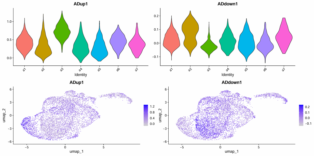
> score_tab
# A tibble: 7 × 5
  sle_reso mean_up mean_down delta     n
  <chr>      <dbl>     <dbl> <dbl> <int>
1 a3         0.732  -0.0217  0.753   630
2 a6         0.451  -0.00553 0.457   401
3 a1         0.415   0.0253  0.389  2841
4 a7         0.370   0.0467  0.323   112
5 a4         0.317   0.0135  0.303   476
6 a5         0.275   0.00709 0.268   429
7 a2         0.321   0.0756  0.246  1542

Up：a3/a6，a1候选
Down：a2，a7候选
No change：a4/a5/a7（mean_up和mean_down没有特别高，delta也不是特别大）

全部数据：

跟着教程做复现_GSE157827_28

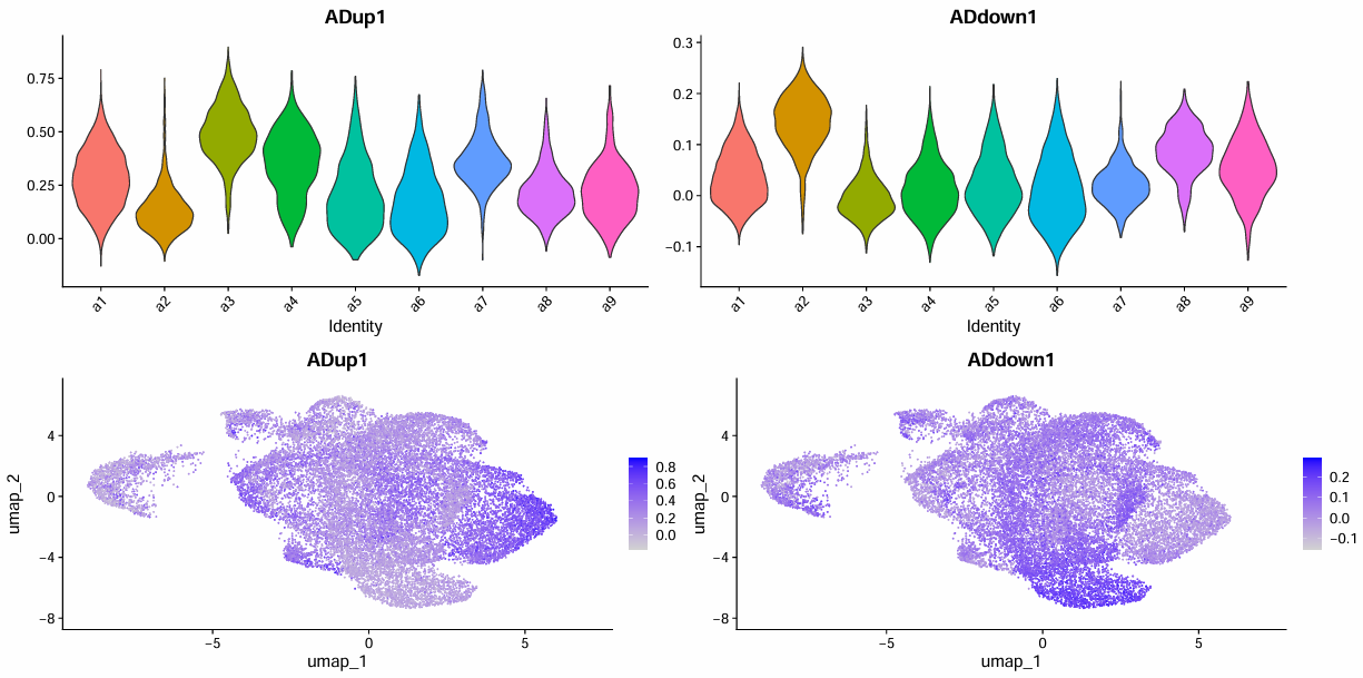
> score_tab
# A tibble: 9 × 5
  sle_reso mean_up mean_down    delta     n
  <chr>      <dbl>     <dbl>    <dbl> <int>
1 a3         0.491  -0.00481  0.496    2445
2 a7         0.367   0.0218   0.345    1059
3 a4         0.349   0.0116   0.338    1414
4 a1         0.283   0.0375   0.246    7043
5 a5         0.202   0.0227   0.179    1394
6 a9         0.223   0.0545   0.168     550
7 a6         0.174   0.0114   0.162    1321
8 a8         0.218   0.0855   0.132     854
9 a2         0.137   0.143   -0.00547  3040

Up：a3/a7/a4，a1候选
Down：a2
No change：a5/a6/a8/a9

# 根据上述结论来分组（为了让后面的图更好看，只有了明显的up和down）
up_core   <- c("a3","a6")
down_core <- c("a2")
# up_core   <- c("a3","a7","a4")
# down_core <- c("a2")
scRNA_astro$subpop <- "No change"
scRNA_astro$subpop[scRNA_astro$sle_reso %in% up_core]   <- "Up"
scRNA_astro$subpop[scRNA_astro$sle_reso %in% down_core] <- "Down"
scRNA_astro$subpop <- factor(scRNA_astro$subpop, levels=c("Up","Down","No change"))
table(scRNA_astro$subpop)
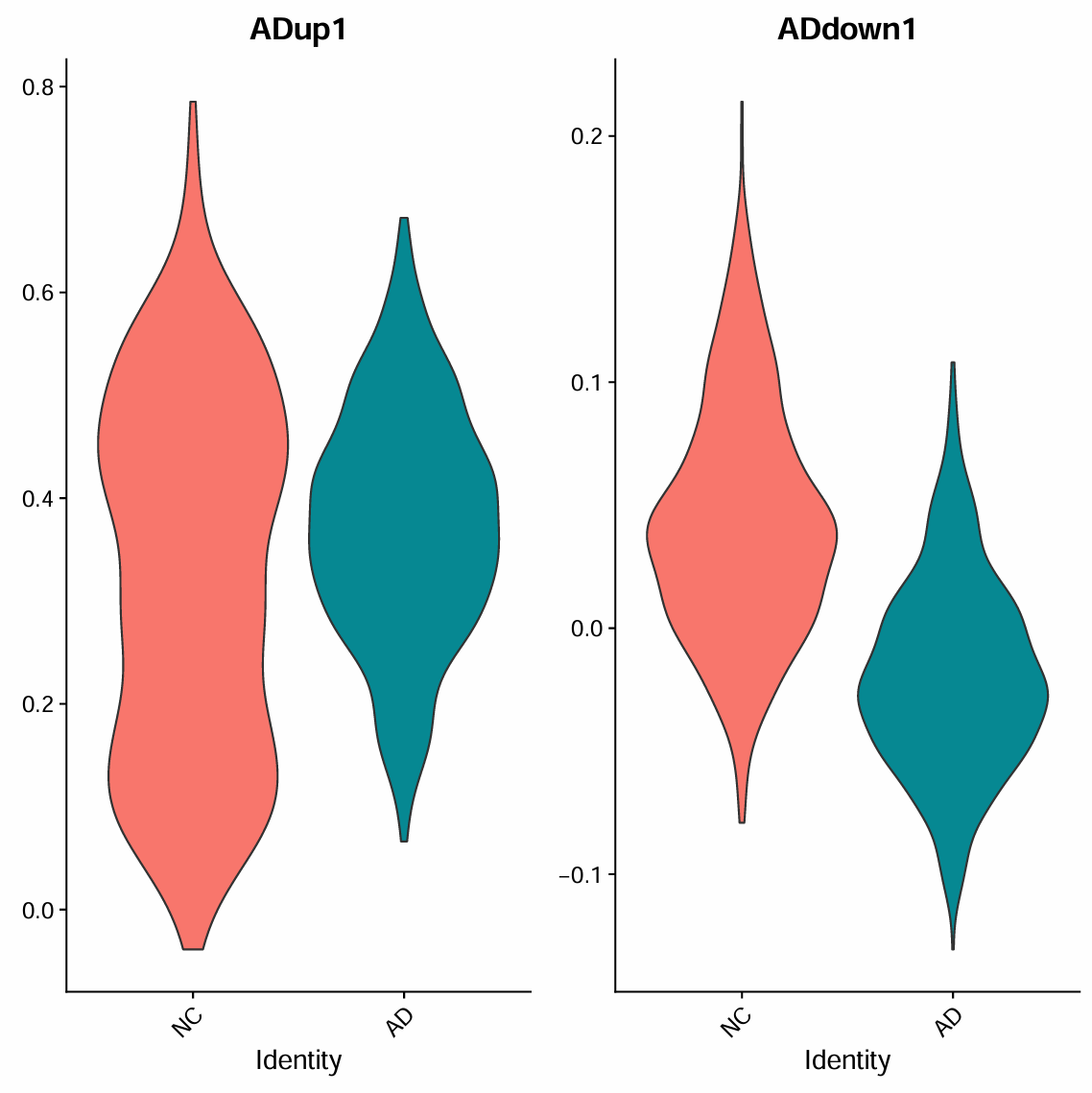
# 确认一下up和down没反（正确：up在AD里富集，down在NC里富集）
prop <- prop.table(table(scRNA_astro$sle_reso, scRNA_astro$group), 1)
prop[c(up_core, down_core), ]

抽样数据的结果比较正常，全部数据的有点奇怪：

> table(scRNA_astro$subpop)

       Up      Down No change 
     4918      3040     11162 
> prop[c(up_core, down_core), ]
    
             NC         AD
  a3 0.10143149 0.89856851
  a7 0.17658168 0.82341832
  a4 0.50000000 0.50000000
  a2 0.91052632 0.08947368

a4这个簇的NC和AD都是0.5，再看一下具体的差异基因信号

pdf(file.path(res_dir, "astro_a4_test.pdf"), width = 8, height = 8)
p <- VlnPlot(scRNA_astro, features = c("ADup1","ADdown1"),
        group.by = "group", split.by = "group",
        idents = "a4", pt.size = 0)
print(p)
dev.off()

跟着教程做复现_GSE157827_29

> table(scRNA_astro$sle_reso, scRNA_astro$group)["a4", ] 
NC AD 
707 707

感觉信号都不明显，up还是不算a4了（更像“稳定的基础Astro状态”，只是其中一些与NC相关的基因程序在AD里下降，但它本身并不在AD中扩张）

# fig_4b
fig_4b <- DimPlot(
  scRNA_astro, 
  group.by = "subpop",
  cols = c("Up"="#e41a1c","Down"="#4daf4a","No change"="#d9d9d9")
)
# 只保留Up/Down
scRNA_astro_sub <- subset(scRNA_astro, subset = subpop != "No change")
# 保存数据
saveRDS(
    scRNA_astro_sub, 
    file = file.path("C:\\Users\\17185\\Desktop\\hERV_calc\\GSE157827\\data", "GSE157827_astro_sub.rds"), 
    compress = "xz"
)

找Up-Down的差异基因并GO富集

scRNA_astro_sub$subpop <- factor(scRNA_astro_sub$subpop, levels = c("Down","Up"))
# Down-Up：avg_log2FC>0表示在Down更高，<0表示在Up更高
marker_Astro <- FindMarkers(
  scRNA_astro_sub, 
  group.by = "subpop",
  ident.1 = "Down", 
  ident.2 = "Up"
)
marker_Astro <- marker_Astro[order(marker_Astro$p_val_adj, decreasing = F), ]
marker_Astro_sig <-  marker_Astro %>%
  rownames_to_column("gene") %>%
  filter(p_val_adj < 0.05, abs(avg_log2FC) >= 0.25) %>% 
  filter(pct.1 >= 0.1 | pct.2 >= 0.1) %>% 
  filter(!grepl("^(ENSG|MT-|LINC)|^(AC|AL)[0-9]", gene))  # 过滤奇奇怪怪的基因
# Down子群体更高表达的基因
top_down <- marker_Astro_sig %>%
  filter(avg_log2FC > 0) %>%
  arrange(p_val_adj, desc(abs(avg_log2FC))) %>%
  slice_head(n = 20) %>%
  pull(gene)
scRNA_astro_sub <- ScaleData(
  scRNA_astro_sub, 
  features = top_down,
  vars.to.regress = c("nFeature_RNA","percent_mito")
)
# fig_4c
fig_4c <- DoHeatmap(
  scRNA_astro_sub, 
  features = top_down,
  group.by = "subpop",
  group.colors = c("Down"="#4daf4a","Up"="#e41a1c"),
  angle = 0
)

GO富集：对所有p值<0.05和log2FC>0.25的基因

# 在down组中差异显著的基因
genes_down <- subset(marker_Astro_sig, avg_log2FC > 0)$gene
# 设置背景：在astro子集里表达过的基因
expr <- GetAssayData(scRNA_astro_sub, slot = "counts")
universe <- rownames(expr)[Matrix::rowSums(expr > 0) >= 10]
# GO富集
ego_down <- enrichGO(
  genes_down[1:300], 
  universe = universe,
  keyType = "SYMBOL", 
  OrgDb = org.Hs.eg.db, 
  ont = "BP",
  pAdjustMethod = "BH",
  pvalueCutoff = 1,
  qvalueCutoff = 1
)
# 取原文中的通路
res <- ego_down@result
interest_go <- which(
  rownames(res) %in% 
    c(
      "GO:0021953","GO:0050769","GO:0021872","GO:0021879",
      "GO:0007409","GO:0042552","GO:0008366","GO:0030900"
    )
)
interest_go <- res$Description[interest_go]
fig_4d <- barplot(ego_down, showCategory=interest_go, cols="pvalue")
# 原始结果
go_res <- barplot(ego_down, showCategory=8, cols="pvalue")
# 保存
pdf(file.path(res_dir, "astro_fig4A-D.pdf"), width = 16, height = 16)
p <- (fig_4a + fig_4b) / (fig_4c + fig_4d) +
  plot_layout(widths = c(2, 1)) +
  plot_annotation(tag_levels = "A")
print(p)
dev.off()
pdf(file.path(res_dir, "astro_go_res.pdf"), width = 8, height = 8)
print(go_res)
dev.off()

跟着教程做复现_GSE157827_30

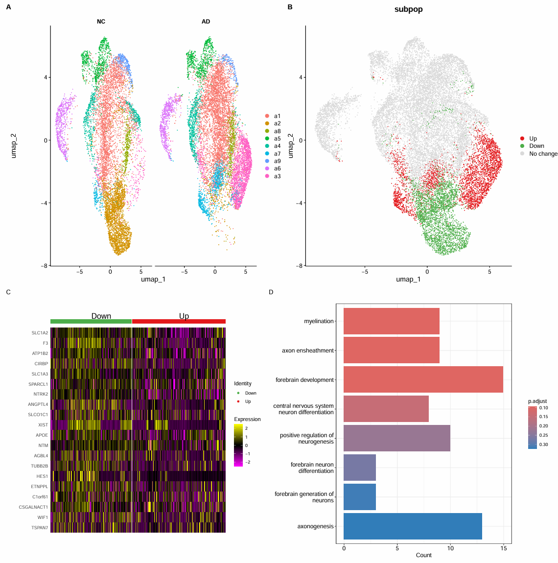
fig_4a：看哪些子簇在AD-NC中明显更常见（比如某些簇在AD中更密）
fig_4b：把很多个Astro子簇合并成3类状态，可以观察up（红）、down（绿）和no change（灰）集中在哪些区域、是否占多数
fig_4c：Down-Up的差异基因（Down高表达）
fig_4d：在富集结果中选一些通路（根据论文）

真实的GO富集结果：

跟着教程做复现_GSE157827_31

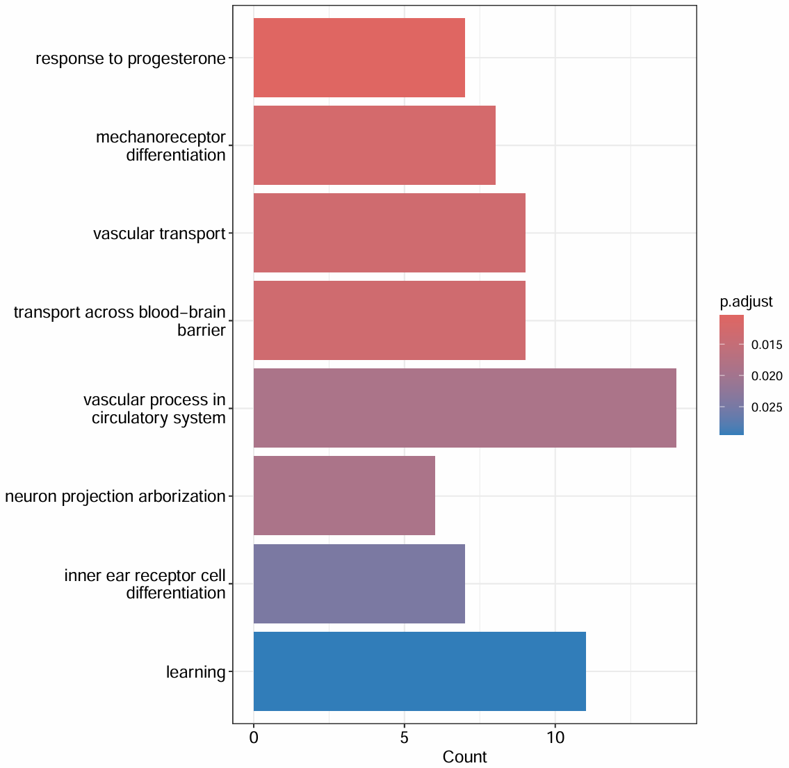
inner ear receptor cell differentiation/learning：因为GO是按“基因注释集合”命名的，如果基因集中恰好包含了某些在该term里出现的基因（哪怕这些基因在脑里的astro也表达），富集就可能把这个term拉出来，并不一定真的说明我的astro是inner ear细胞
vascular/blood-brainbarrier/transport/response to progesterone（血管过程、跨 BBB 运输、血管运输、激素反应）：提示脑血管单元相关状态变化

down/up聚类是什么意思：在astro这个大类里面，找到与AD相关变化最明显的亚状态

down/up不是指某个单基因上调/下调，而是指某一簇astro的整体转录特征更像AD相关上调/下调的方向
我们是如何划分这个聚类的：
- 先得到在astro里AD-NC的差异表达基因（使用前面的all_markers_sig$Astro）
- 在给每个细胞计算分数：score_up是AD_up_genes的综合表达强度，score_down是AD_down_genes的综合表达强度
- 计算每个astro子聚类的平均score_up（mean_up）和平均score_down（mean_down），以及它们的差值（delta）
- 根据这些值来将每个子聚类归到up/down/no change组
为什么要分组而不是像最早一样直接做AD-NC的差异分析：
- astro里面可能只有一小部分状态在AD中发生明显变化；把所有astro混在一起做DE，会把信号稀释掉
- 某些astro状态上调某条通路，另一些状态下调同一条通路，混起来做DE可能看不到任何显著结果

一些小讨论

细胞轨迹

需要的数据：

同一生物过程的连续状态（比如分化、激活、退化、应激反应的渐变），而不是“完全离散的几团细胞”
足够的细胞数（每条潜在分支上都要有覆盖）
RNA velocity：需要把reads分成“落在外显子（spliced）”和“落在内含子（unspliced）”两类

在AD分析中：

轨迹通常指“微胶质/星形胶质细胞等的激活/反应性连续谱”（而不是发育分化那种“真实时间序列”）
选定一个时间来作为轨迹的坐标
- 真实/外部时间(external time)：Braak tangle stage、CERAD、临床分期、年龄，这些都是“样本层面的标签”，不是从表达里推出来的
因为一个样本只有一个braak分期，所以要把AD+NC的不同分期的样本合在一起
- 伪时间(pseudotime)：从细胞表达/可及性结构里推出来的“状态排序”，描述同一细胞类型内部从“稳态→反应态/炎症态/应激态…”的连续变化
pseudotime只给顺序，不保证方向因果：只能找到一条“连续变化的主路径”，然后把细胞按在路径上的位置排个序。但同一条路径，反过来也成立，必须人为指定起点；而且“变化顺序”相近，只能说明“这些细胞状态彼此更像、更平滑过渡”，并不等价于“细胞真的按这个顺序发生变化”，更不等价于“疾病导致了这个变化”

常用工具：

经典pseudotime（只给顺序，不保证方向因果）：Monocle3、Slingshot、Scanpy(PAGA/DPT)、Palantir
带“方向”的动力学（推测哪些是起始态、哪些是终末态、以及每个细胞走向各终末态的概率）：scVelo、CellRank
轨迹上的差异表达/比较（比较AD和NC在轨迹上是否不同步/不同形态）：tradeSeq

大体思路：

选一个细胞类型/亚群，比如microglia或astrocyte，通常状态连续性更强
在该子集上做降维/邻接图
Monocle3/Slingshot进行pseudotime/trajectory
把“对照/Braak分期较早”富集的那端作为起点
把关心的变量投到轨迹上看趋势，比如HERV_fraction、某几个关键hERV位点的表达量、某几个关键基因模块分数
比较“AD-Ctrl的细胞在pseudotime上的分布是否整体偏移”、“同一pseudotime区间内，AD-Ctrl的表达曲线是否不同”（tradeSeq）、“不同braak分期的细胞在pseudotime上的富集点是否逐级移动”

注意：

不是“按Braak划分时间再去建轨迹”，而是“先从细胞状态结构里建轨迹，再用Braak去解释这条轴到底像不像疾病进展”
当有足够多的分期层级、每个分期有多个样本、取样脑区相对一致时，我们才选用braak分期作为时间轴

表观遗传相关

染色质状态的漂移/侵蚀(epigenetic drift/erosion)：抑制性异染色质维护变差，导致本应沉默的重复序列/TE更容易被激活，同时一些原本稳定表达的程序可能被破坏

需要的数据：

scATAC-seq/Multiome：用开放染色质(ATAC)作为抑制/激活的判断标准
H3K9me3/H3K27me3（经典抑制性标记）的ChIP-seq，或更适合单细胞/低量的CUT&Tag/CUT&RUN
bulk WGBS/RRBS或单细胞甲基化（公共数据较少）

在单细胞分析中：

scATAC与多模态分析：Signac（更适配Seurat）、ArchR
scRNA+scATAC：直接用Seurat的scRNA–scATAC integration流程（无论同细胞multiome，还是不同细胞但同体系的ATAC+RNA）
把细胞轨迹延伸到染色质层面：Signac+Monocle3+scATAC数据

hERV位点的“染色质状态”怎么量化：即“这个hERV附近（或这个TE本体）在某类细胞里，是更开放还是更被压制”

从gtf中获取每个hERV位点的坐标
对每个位点，取它周围例如±2kb/±5kb的ATAC峰（尤其是可唯一比对的峰）
- ATAC峰：“开放染色质区域”的候选集合（常见于启动子、增强子等调控元件附近）
以“这些峰的可及性(peak accessibility)”作为“这个TE的染色质更开放/更关闭”的标志
- peak accessibility：某个细胞在某个peak上的信号强弱
还可以结合H3K9me3、H3K27me3这类抑制性表观标记
- ATAC是说某块染色质是否开放，H3K9me3/H3K27me3是说某块染色质有没有抑制性标记，两者结合起来就更完整