使用我的GSE157827数据进行初步分析
other-other2025.12.31-2026.1.14研究进展
try1
构建Seurat对象
library(Seurat)
library(Matrix)
library(tidyverse)
library(readxl)
# 读取计数矩阵
data_root <- "/public/home/GENE_proc/wth/GSE157827/mtx/"
read_one_srr <- function(srr) {
  gene_dir <- file.path(data_root, srr, "gene")
  herv_dir <- file.path(data_root, srr, "hERV")
  gene_counts <- ReadMtx(
    mtx = file.path(gene_dir, "counts.mtx"),
    features = file.path(gene_dir, "features.tsv"),
    cells = file.path(gene_dir, "barcodes.tsv")
  )
  herv_counts <- ReadMtx(
    mtx = file.path(herv_dir, "counts.mtx"),
    features = file.path(herv_dir, "features.tsv"),
    cells = file.path(herv_dir, "barcodes.tsv"),
    feature.column = 1
  )
  colnames(gene_counts) <- paste(srr, colnames(gene_counts), sep = "_")
  colnames(herv_counts) <- paste(srr, colnames(herv_counts), sep = "_")
  common_cells <- intersect(colnames(gene_counts), colnames(herv_counts))
  gene_counts <- gene_counts[, common_cells, drop = FALSE]
  herv_counts <- herv_counts[, common_cells, drop = FALSE]
  seu <- CreateSeuratObject(
    counts = gene_counts,
    assay = "RNA",
    project = "AD_hERV"
  )
  seu[["HERV"]] <- CreateAssayObject(counts = herv_counts)
  seu$SRR_id <- srr
  return(seu)
}
srr_ids <- list.dirs(data_root, full.names = FALSE, recursive = FALSE)
seu_list <- list()
for (srr in srr_ids) {
  seu <- read_one_srr(srr)
  if (!is.null(seu)) {
    seu_list[[srr]] <- seu
  }
}
seu <- Reduce(function(x, y) merge(x, y), seu_list)
rm(seu_list)
head(seu@meta.data)
# 添加metadata
meta_map <- read_xlsx("/public/home/GENE_proc/wth/GSE157827/raw_data/metadata/metadata.xlsx")
sample_info <- read_xlsx("/public/home/GENE_proc/wth/GSE157827/raw_data/metadata/sample_info.xlsx")
names(meta_map) <- make.names(names(meta_map))
names(sample_info) <- make.names(names(sample_info))
meta_map <- meta_map %>%
  select(individuals, SRR_id, sample_id, tissue)
colnames(meta_map) <- c("sample_id", "SRR_id", "GSM", "tissue")
metadata <- meta_map %>%
  left_join(sample_info, by = "sample_id")
cell_meta <- seu@meta.data %>%
  rownames_to_column("cell")
cell_meta2 <- cell_meta %>%
  left_join(metadata, by = "SRR_id")
sum(is.na(cell_meta2$sample_id))  # 检查是否有映射失败
new_cols <- setdiff(names(cell_meta2), names(seu@meta.data))
meta_to_add <- cell_meta2 %>%
  select(cell, all_of(new_cols)) %>%
  column_to_rownames("cell")
seu <- AddMetaData(seu, metadata = meta_to_add)
# 合并每个layers
seu <- JoinLayers(seu, assay = "RNA")
Layers(seu, assay = "RNA")  # 检查一下layers
# 线粒体/核糖体比例
seu <- PercentageFeatureSet(seu, pattern = "^MT-", col.name = "percent_mito")
seu <- PercentageFeatureSet(seu, pattern = "^RP[SL]", col.name = "percent_ribo")
# 保存数据
saveRDS(
  seu,
  file = "/public/home/GENE_proc/wth/GSE157827/my_data/GSE157827.rds",
  compress = "xz"
)
> seu
An object of class Seurat
93660 features across 304953 samples within 2 assays
Active assay: RNA (78691 features, 0 variable features)
 1 layer present: counts
 1 other assay present: HERV
质控
看数据分布
scRNA <- readRDS("/public/home/GENE_proc/wth/GSE157827/my_data/GSE157827.rds")
res_dir <- "/public/home/GENE_proc/wth/GSE157827/res/"
scRNA$orig.ident <- scRNA$sample_id
scRNA$group <- factor(scRNA$diagnosis, levels = c("NC", "AD"))
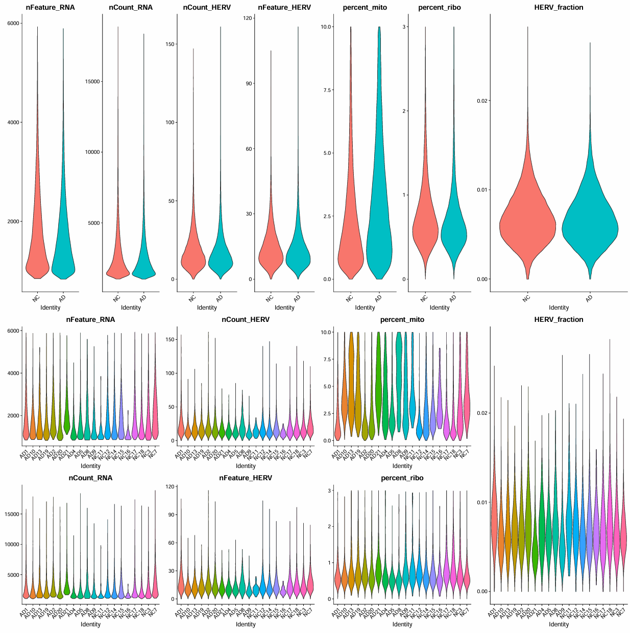
# 基因数/UMI数
feats <- c("nFeature_RNA", "nCount_RNA")
p_filt_b_1 <- VlnPlot(
scRNA, features = feats,
pt.size = 0,
ncol = 2,
group.by = "group"
) + NoLegend()
p_filt_b_2 <- VlnPlot(
scRNA, features = feats,
pt.size = 0,
ncol = 1,
group.by = "orig.ident"
) + NoLegend()
# HERV数
feats <- c("nCount_HERV", "nFeature_HERV")
p_filt_b_3 <- VlnPlot(
scRNA, features = feats,
pt.size = 0,
ncol = 2,
group.by = "group"
) + NoLegend()
p_filt_b_4 <- VlnPlot(
scRNA, features = feats,
pt.size = 0,
ncol = 1,
group.by = "orig.ident"
) + NoLegend()
# HERV占整个转录本的比例
scRNA$HERV_fraction <- scRNA$nCount_HERV / (scRNA$nCount_HERV + scRNA$nCount_RNA)
p_filt_b_7 <- VlnPlot(
scRNA, features = "HERV_fraction",
pt.size = 0,
ncol = 1,
group.by = "group"
) + NoLegend()
p_filt_b_8 <- VlnPlot(
scRNA, features = "HERV_fraction",
pt.size = 0,
ncol = 1,
group.by = "orig.ident"
) + NoLegend()
# 线粒体/核糖体比例
feats <- c("percent_mito", "percent_ribo")
p_filt_b_5 <- VlnPlot(
scRNA, features = feats,
pt.size = 0,
ncol = 2,
group.by = "group" # 按AD/NC分组看分布
) + NoLegend()
p_filt_b_6 <- VlnPlot(
scRNA, features = feats,
pt.size = 0,
ncol = 1,
group.by = "orig.ident" # 按样本看分布
) + NoLegend()
# 拼图展示
pdf(file.path(res_dir, "before_filter.pdf"), width = 20, height = 20)
p <- (p_filt_b_1 / p_filt_b_2) | (p_filt_b_3 / p_filt_b_4) | (p_filt_b_5 / p_filt_b_6) | (p_filt_b_7 / p_filt_b_8)
print(p)
dev.off()
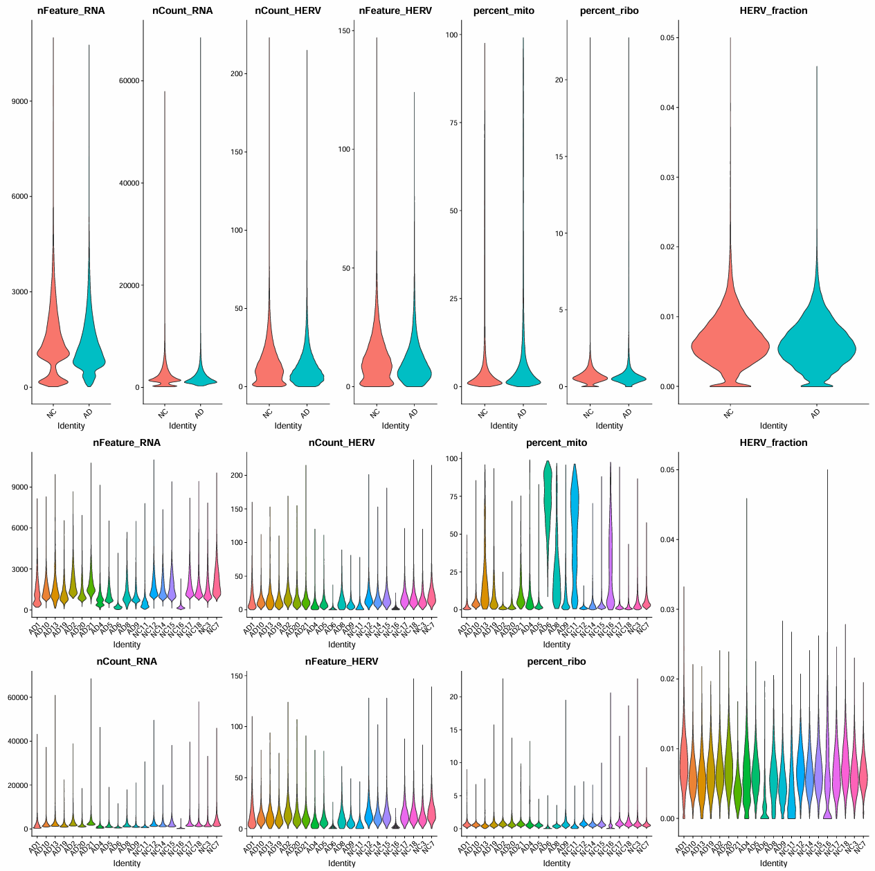
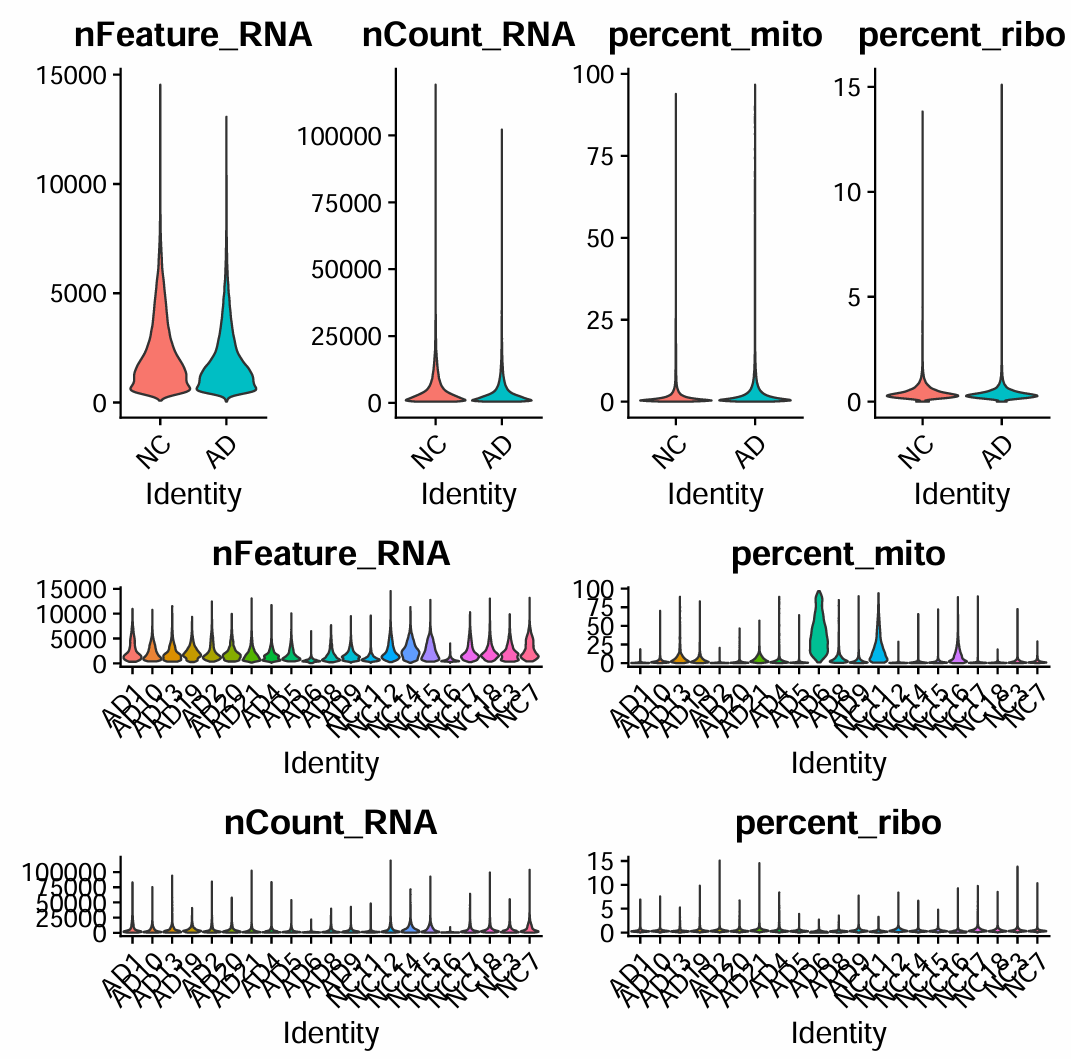
> summary(scRNA$nFeature_RNA)
   Min. 1st Qu.  Median    Mean 3rd Qu.    Max.
     16     799    1203    1414    1854   10993
> summary(scRNA$nCount_RNA)
   Min. 1st Qu.  Median    Mean 3rd Qu.    Max.
    144    1099    1662    2239    2728   68430
> summary(scRNA$nCount_HERV)
   Min. 1st Qu.  Median    Mean 3rd Qu.    Max.
   0.00    5.00   11.00   14.07   19.00  223.00
> summary(scRNA$nFeature_HERV)
   Min. 1st Qu.  Median    Mean 3rd Qu.    Max.
   0.00    5.00    9.00   11.46   15.00  147.00
> summary(scRNA$HERV_fraction)
    Min.  1st Qu.   Median     Mean  3rd Qu.     Max.
0.000000 0.004047 0.006073 0.006409 0.008417 0.050000
> summary(scRNA$percent_mito)
   Min. 1st Qu.  Median    Mean 3rd Qu.    Max.
  0.000   1.382   3.100  10.467   8.076  99.093
> summary(scRNA$percent_ribo)
   Min. 1st Qu.  Median    Mean 3rd Qu.    Max.
 0.0000  0.4058  0.5969  0.7382  0.8642 22.7354
确定过滤阈值
细胞阈值:
# 过滤阈值
retained_c_umi_low <- scRNA$nFeature_RNA > 900
retained_c_umi_high <- scRNA$nFeature_RNA < 6000
retained_c_count_low <- scRNA$nCount_RNA > 1200
retained_c_count_high <- scRNA$nCount_RNA < 30000
retained_c_mito <- scRNA$percent_mito < 10
retained_c_ribo <- scRNA$percent_ribo < 3
keep_cells <- retained_c_umi_low & retained_c_umi_high & retained_c_mito & retained_c_ribo
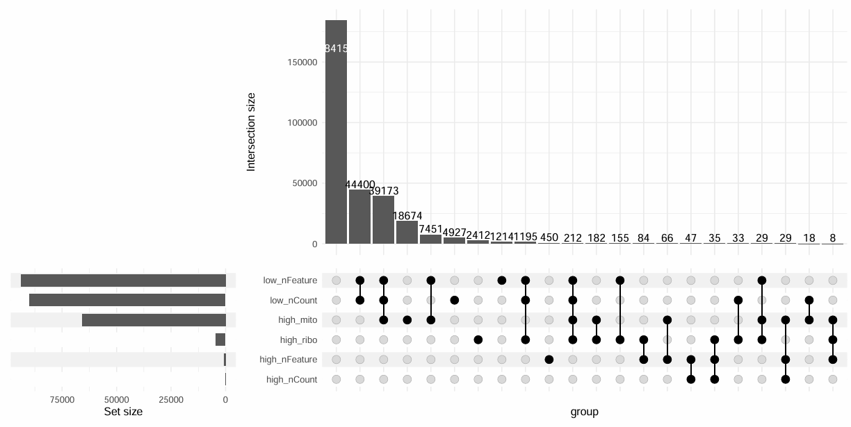
# 看看交集
df_fail <- data.frame(
cell = Cells(scRNA),
low_nFeature = !retained_c_umi_low,
high_nFeature = !retained_c_umi_high,
low_nCount = !retained_c_count_low,
high_nCount = !retained_c_count_high,
high_mito = !retained_c_mito,
high_ribo = !retained_c_ribo
)
pdf(file.path(res_dir, "cell_filter_upset.pdf"), width = 12, height = 6)
ComplexUpset::upset(
df_fail,
intersect = c("low_nFeature","high_nFeature","low_nCount","high_nCount","high_mito","high_ribo"),
base_annotations = list('Intersection size' = intersection_size())
)
dev.off()
基因阈值:
scRNA_cells <- subset(scRNA, cells = Cells(scRNA)[keep_cells])
counts_rna <- GetAssayData(scRNA_cells, assay = "RNA", slot = "counts")
feature_rowsum <- Matrix::rowSums(counts_rna > 0)
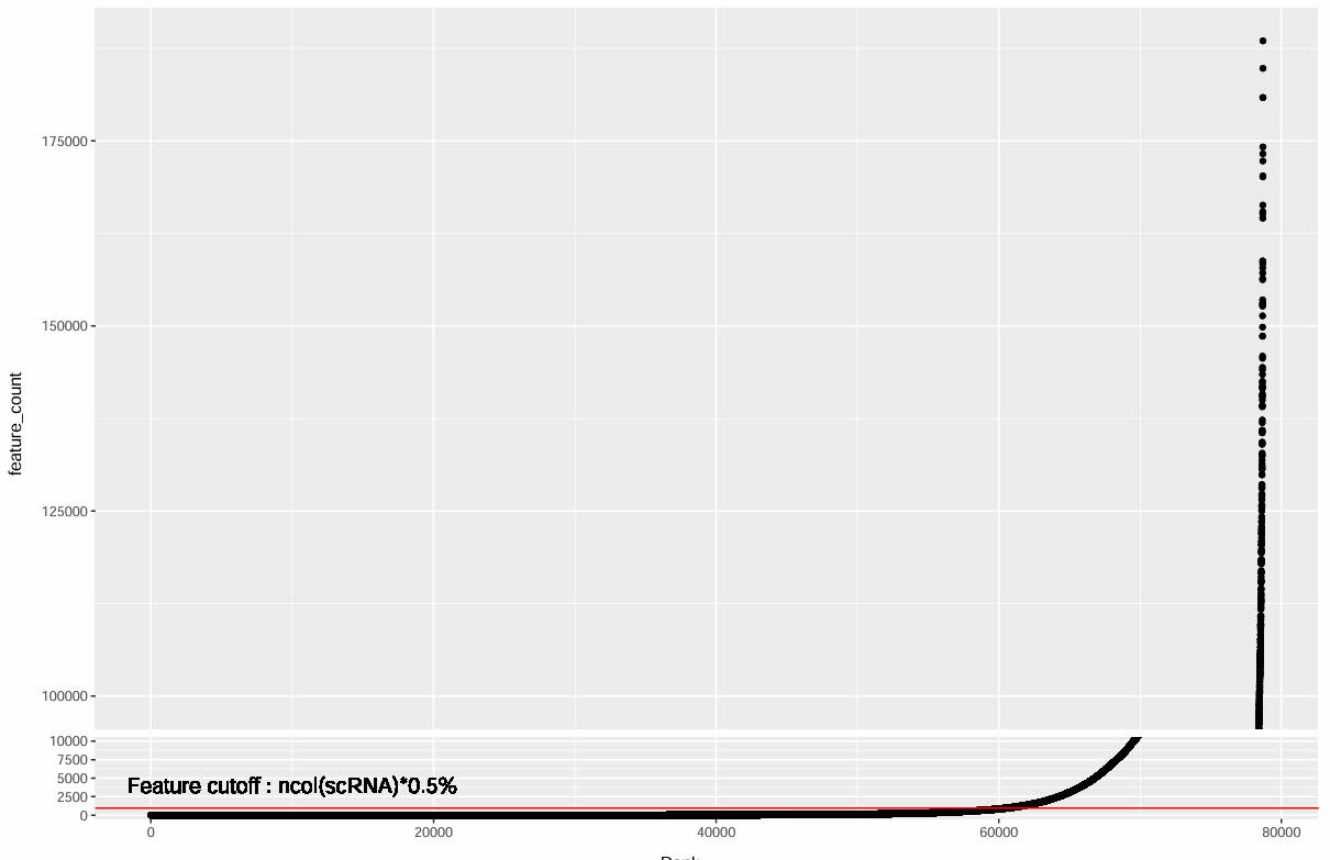
retained_f_low <- feature_rowsum > ncol(scRNA_cells) * 0.005 # 只保留“至少在0.5%细胞里表达过”的基因
genes_keep <- names(feature_rowsum)[retained_f_low]
# rankplot辅助看阈值
rankplot <- data.frame(
feature_count = sort(feature_rowsum),
gene = names(sort(feature_rowsum)),
Rank = seq_along(feature_rowsum)
)
library(ggbreak)
pdf(file.path(res_dir, "gene_filter.pdf"), width = 12, height = 8)
p_gene <- ggplot(rankplot, aes(x = Rank, y = feature_count)) +
geom_point() +
scale_y_break(c(10000, 100000)) +
geom_hline(yintercept = ncol(scRNA_cells) * 0.005, color = "red") +
geom_text(x = 10000, y = 4000, size = 5,
label = "Feature cutoff : ncol(scRNA)*0.5%")
print(p_gene)
dev.off()
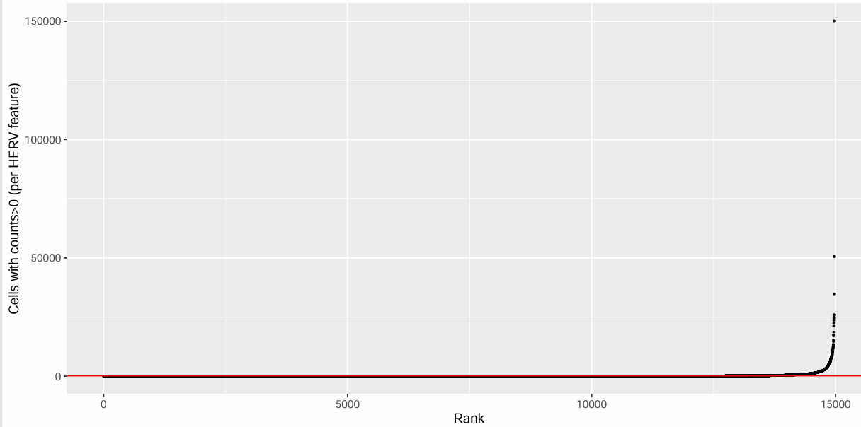
hERV阈值:
counts_herv <- GetAssayData(scRNA_cells, assay = "HERV", slot = "counts")
herv_rowsum <- Matrix::rowSums(counts_herv > 0)
herv_keep <- names(herv_rowsum)[herv_rowsum > 50]  # 至少50个细胞中表达过
cat("HERV features before:", nrow(counts_herv), "\n")  # 14969
cat("HERV features kept:", length(herv_keep), "\n")  # 3351
rankplot_herv <- data.frame(
  feature_count = sort(herv_rowsum),
  feature = names(sort(herv_rowsum)),
  Rank = seq_along(herv_rowsum)
)
pdf(file.path(res_dir, "gene_filter_herv.pdf"), width = 10, height = 5)
ggplot(rankplot_herv, aes(x = Rank, y = feature_count)) +
  geom_point(size = 0.4) +
  geom_hline(yintercept = herv_cutoff, color = "red") +
  xlab("Rank") + ylab("Cells with counts>0 (per HERV feature)")
dev.off()
过滤
scRNA_cells[["RNA"]] <- subset(scRNA_cells[["RNA"]], features = genes_keep)
scRNA_cells[["HERV"]] <- subset(scRNA_cells[["HERV"]], features = herv_keep)
# 重新计算nCount和nFeature
rna_counts <- GetAssayData(scRNA_cells, assay = "RNA", slot = "counts")
scRNA_cells$nCount_RNA <- Matrix::colSums(rna_counts)
scRNA_cells$nFeature_RNA <- Matrix::colSums(rna_counts > 0)
herv_counts <- GetAssayData(scRNA_cells, assay = "HERV", slot = "counts")
scRNA_cells$nCount_HERV <- Matrix::colSums(herv_counts)
scRNA_cells$nFeature_HERV <- Matrix::colSums(herv_counts > 0)
scRNA_cells$HERV_fraction <- scRNA_cells$nCount_HERV / (scRNA_cells$nCount_HERV + scRNA_cells$nCount_RNA)
# 查看过滤后分布
# 基因数/UMI数
feats <- c("nFeature_RNA", "nCount_RNA")
p_filt_a_1 <- VlnPlot(
  scRNA_cells, features = feats,
  pt.size = 0,
  ncol = 2,
  group.by = "group"
) + NoLegend()
p_filt_a_2 <- VlnPlot(
  scRNA_cells, features = feats,
  pt.size = 0,
  ncol = 1,
  group.by = "orig.ident"
) + NoLegend()
# HERV数
feats <- c("nCount_HERV", "nFeature_HERV")
p_filt_a_3 <- VlnPlot(
  scRNA_cells, features = feats,
  pt.size = 0,
  ncol = 2,
  group.by = "group"
) + NoLegend()
p_filt_a_4 <- VlnPlot(
  scRNA_cells, features = feats,
  pt.size = 0,
  ncol = 1,
  group.by = "orig.ident"
) + NoLegend()
p_filt_a_7 <- VlnPlot(
  scRNA_cells, features = "HERV_fraction",
  pt.size = 0,
  ncol = 1,
  group.by = "group"
) + NoLegend()
p_filt_a_8 <- VlnPlot(
  scRNA_cells, features = "HERV_fraction",
  pt.size = 0,
  ncol = 1,
  group.by = "orig.ident"
) + NoLegend()
# 线粒体/核糖体比例
feats <- c("percent_mito", "percent_ribo")
p_filt_a_5 <- VlnPlot(
  scRNA_cells, features = feats,
  pt.size = 0,
  ncol = 2,
  group.by = "group"  # 按AD/NC分组看分布
) + NoLegend()
p_filt_a_6 <- VlnPlot(
  scRNA_cells, features = feats,
  pt.size = 0,
  ncol = 1,
  group.by = "orig.ident"  # 按样本看分布
) + NoLegend()
# 拼图展示
pdf(file.path(res_dir, "after_filter.pdf"), width = 20, height = 20)
p <- (p_filt_a_1 / p_filt_a_2) | (p_filt_a_3 / p_filt_a_4) | (p_filt_a_5 / p_filt_a_6) | (p_filt_a_7 / p_filt_a_8)
print(p)
dev.off()
# 保存数据
saveRDS(
    scRNA_cells,
    file = "/public/home/GENE_proc/wth/GSE157827/my_data/GSE157827_filt.rds",
    compress = "xz"
)
> dim(scRNA_cells)
[1]  18217 189086
> table(scRNA_cells$group)
    NC     AD
100788  88298
> table(scRNA_cells$orig.ident)
  AD1  AD10  AD13  AD19   AD2  AD20  AD21   AD4   AD5   AD8   AD9  NC11  NC12
 9802 19632  1128  4623 14677 11959  3708  3147 11639   592  7391   171 18635
 NC14  NC15  NC16  NC17  NC18   NC3   NC7
18437 13877   133 16229 14671  8078 10557
可以看到似乎有的样本细胞数非常少,不过查看作者的计数矩阵,似乎也是有一些样本的细胞数很少。我的结果中AD8、NC11、NC16在作者的计数矩阵中也是属于比较少的一堆,而且我设置的阈值比作者的更严格,所以细胞数就更少了
> table(author_scRNA$orig.ident)
  NC3   NC7  NC11  NC12  NC14  NC15  NC16  NC17  NC18   AD1   AD2   AD4   AD5
 6218  6372  1587 15568 10932  8385  4235 14263 11476  6173 15276  5980 12356
  AD6   AD8   AD9  AD10  AD13  AD19  AD20  AD21
  311  2405  9789 16013  1608  3614  9169  7786
与作者的计数矩阵对照
library(Matrix)
seu_ours <- readRDS("/public/home/GENE_proc/wth/GSE157827/my_data/GSE157827_filt.rds")
seu_auth <- readRDS("/public/home/GENE_proc/wth/GSE157827/data/GSE157827_filt.rds")
res_dir <- "/public/home/GENE_proc/wth/GSE157827/res/"
seu_ours$orig.ident <- seu_ours$sample_id
seu_ours$group <- factor(seu_ours$diagnosis, levels = c("NC", "AD"))
meta_ours <- seu_ours@meta.data %>%
  rownames_to_column("cell_ours")
meta_ours <- meta_ours %>%
  mutate(
    barcode = str_replace(cell_ours, "^.*_", ""),
    GSM = as.character(GSM),
    sample = as.character(orig.ident),
    cell_like_auth = paste0(GSM, "_", sample, "_", barcode, "-1"),
    cell_like_auth_no1 = str_replace(cell_like_auth, "-1$", "")
  )
auth_cells_raw <- colnames(seu_auth)
auth_cells_no1 <- str_replace(auth_cells_raw, "-1$", "")
our_ids_no1 <- meta_ours$cell_like_auth_no1
# 看看我的细胞和作者的细胞有多少是相同的
common_no1 <- intersect(our_ids_no1, auth_cells_no1)
cat("ours cells:", length(our_ids_no1), "\n")
cat("auth cells:", length(auth_cells_no1), "\n")
cat("common cells:", length(common_no1), "\n")
cat("overlap % (of ours):", round(length(common_no1)/length(our_ids_no1)*100, 2), "%\n")
cat("overlap % (of auth):", round(length(common_no1)/length(auth_cells_no1)*100, 2), "%\n")
很奇怪,这步的重叠率只有大概25%,即使我拿原始计数矩阵也只有大约30%
在重叠的细胞上比较计数的一致性:
mat_ours <- GetAssayData(seu_ours, assay = "RNA", slot = "counts")
mat_auth <- GetAssayData(seu_auth, assay = "RNA", slot = "counts")
our_map <- setNames(meta_ours$cell_ours, meta_ours$cell_like_auth_no1)
our_cells_common <- unname(our_map[common_no1])
auth_map <- setNames(auth_cells_raw, auth_cells_no1)
auth_cells_common <- unname(auth_map[common_no1])
common_genes <- intersect(rownames(mat_ours), rownames(mat_auth))
mat_ours_sub <- mat_ours[common_genes, our_cells_common, drop = FALSE]
mat_auth_sub <- mat_auth[common_genes, auth_cells_common, drop = FALSE]
cat("common genes:", length(common_genes), "\n")
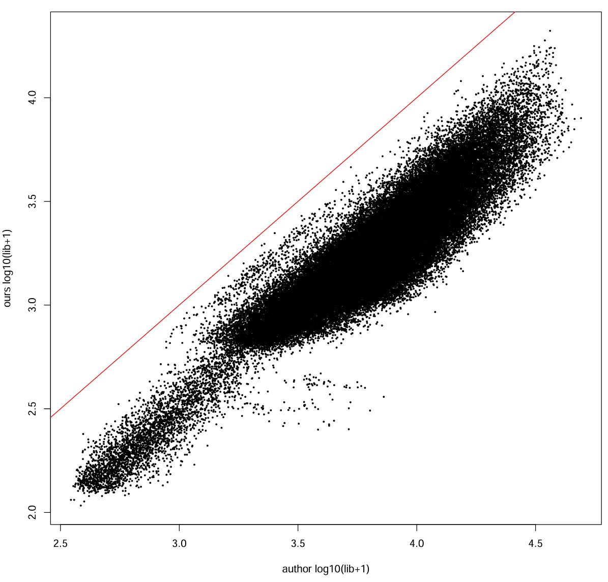
每个细胞的总UMI:
our_lib  <- Matrix::colSums(mat_ours_sub)
auth_lib <- Matrix::colSums(mat_auth_sub)
cor_lib <- cor(log10(our_lib + 1), log10(auth_lib + 1))
cat("cell library size corr (log10+1):", cor_lib, "\n")  # 0.922925
pdf(file.path(res_dir, "author_our_umi.pdf"), width = 10, height = 10)
plot(log10(auth_lib + 1), log10(our_lib + 1),
     xlab = "author log10(lib+1)", ylab = "ours log10(lib+1)", pch = 16, cex = 0.4)
abline(0, 1, col = "red")
dev.off()
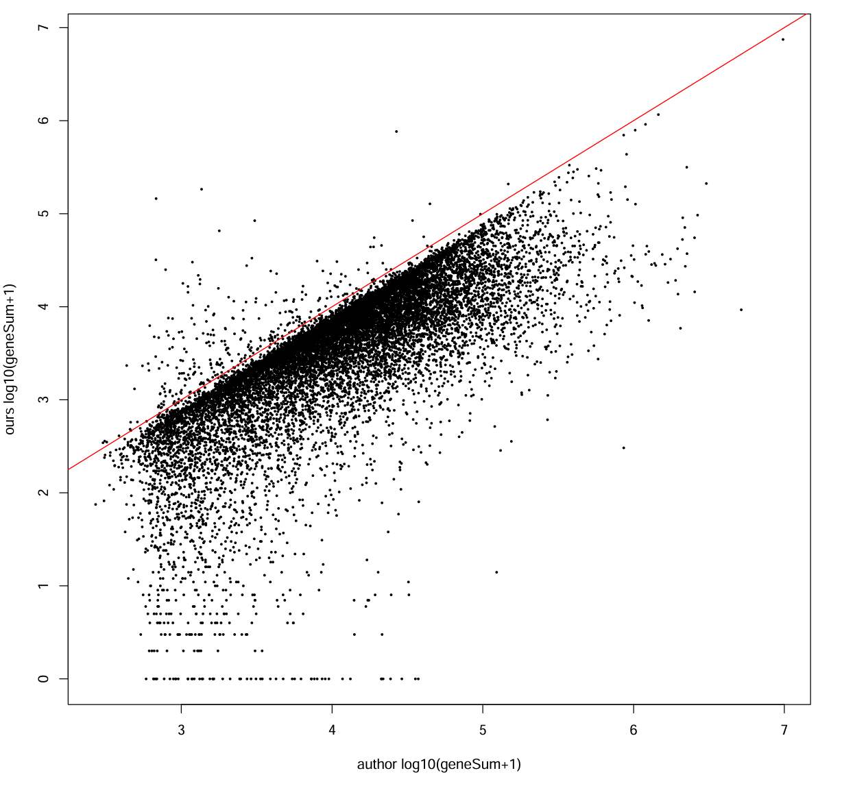
每个基因的总counts:
our_gene_sum  <- Matrix::rowSums(mat_ours_sub)
auth_gene_sum <- Matrix::rowSums(mat_auth_sub)
cor_gene <- cor(log10(our_gene_sum + 1), log10(auth_gene_sum + 1))
cat("gene total counts corr (log10+1):", cor_gene, "\n")  # 0.7527359
pdf(file.path(res_dir, "author_our_counts.pdf"), width = 10, height = 10)
plot(log10(auth_gene_sum + 1), log10(our_gene_sum + 1),
     xlab = "author log10(geneSum+1)", ylab = "ours log10(geneSum+1)", pch = 16, cex = 0.4)
abline(0, 1, col = "red")
dev.off()
每个细胞的基因向量相关性(随机抽一些细胞):
set.seed(1)
k <- min(200, ncol(mat_ours_sub))
cells_pick <- sample(seq_len(ncol(mat_ours_sub)), k)
cors <- sapply(cells_pick, function(j){
  x <- as.numeric(mat_ours_sub[, j])
  y <- as.numeric(mat_auth_sub[, j])
  cor(log1p(x), log1p(y))
})
summary(cors)
pdf(file.path(res_dir, "author_our_corr.pdf"), width = 10, height = 10)
hist(cors, breaks = 30, main = "Per-cell cor(log1p counts)", xlab = "cor")
dev.off()
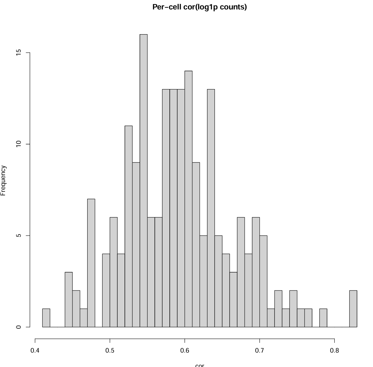
可以看到在重叠的细胞内,我的计数结果和作者的基本一致
为了看一看是什么原因导致细胞名不一致,我又按样本(GSM)分别看了重叠率,发现所有样本的重叠率都在20%-60%区间,没有说某几个样本完全重叠/不重叠的情况,说明barcode不匹配是发生在所有样本上的
询问了GPT,除了之前反复提过的STARsolo和cellranger计数上的区别,很有可能作者提供的计数矩阵和fastq数据不完全匹配——比如一个GSM对应多个SRR(技术重复/不同lane),我是计数了全部SRR,并且最后直接进行合并,作者可能只取了部分/合并时处理方式不同(比如过滤掉某些样本),这也可以解释为什么上面过滤时,我在第一次尝试时,虽然使用了和作者一样(甚至更严格)的阈值,但最后的细胞数却多了近1/3(24w-17w),后面才不得不逐渐提高阈值来让细胞数和作者的接近
为了验证这个想法,我按SRR分组计算重叠率,发现确实在SRR层面,重叠率差异很大,有些接近100%,有些只有30%-5%,这样的结果就很奇怪
之后我又看了“同一个GSM内,一个barcode会不会出现在多个SRR中”,结果发现很多barcode在GSM内出现次数都近似于该GSM包含的SRR数,就是说,这里的每个SRR是同一文库的lane拆分,而我在计数时把它们都当成独立run进行计数了
最后只能重跑一篇计数流程,把属于同一GSM的多个SRR当作多lane输入给STAR
- 不能直接把多个SRR的计数矩阵相加,因为UMI的去重是在计数阶段,直接相加会把跨lane的相同UMI叠加,产生系统性偏差
try2
STAR计数
先做一个SRR->GSM的映射srr2gsm.csv
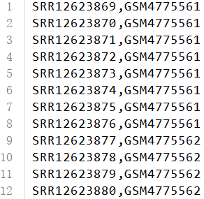
与上一版本的代码相比,除了先把SRR都映射到GSM上
-
--soloUMIlen 10:作者的GSM说明里写的是Chromium Single Cell 3′ Library Kit v3,按理论来讲v3的UMI长度应该是12(官方pdf是这么说的),我之前写成了10,但实测改为12之后反而是错的 -
--soloFeatures Gene GeneFull:打开pre-mRNA计数,后续都用GeneFull中的结果 -
--soloCellFilter EmptyDrops_CR:让cell calling策略接近CellRanger(使用更像CellRanger的细胞筛选方法)
workDir=/public/home/GENE_proc/wth/GSE157827/
genomeDir=/public/home/wangtianhao/Desktop/STAR_ref/hg38/
fqDir=${workDir}/fastq
mapFile=${fqDir}/srr2gsm.csv
whitelist=/public/home/wangtianhao/Desktop/STAR_ref/whitelist/3M-february-2018.txt
hERV_gtf=/public/home/wangtianhao/Desktop/STAR_ref/transcripts.gtf
res_barcodes=barcodes
res_features=features
res_counts=counts
cd ${workDir}
module load miniconda3/base
dos2unix ${mapFile}
# 取所有GSM
GSM_LIST=$(cut -d',' -f2 "${mapFile}" | sort -u)
for GSM in ${GSM_LIST}; do
    GSM=${GSM//$'\r'/}
    echo "=============================="
    echo "[GSM] ${GSM}"
    SRR_LIST=$(awk -F',' -v g="${GSM}" '$2==g{print $1}' "${mapFile}")
    nSRR=$(echo "${SRR_LIST}" | wc -l | awk '{print $1}')
    echo "  SRR count: ${nSRR}"
    echo "${SRR_LIST}" | sed 's/^/  - /'
    cdna_files=$(echo "${SRR_LIST}" | sed "s|^|${fqDir}/|; s|$|_2.fastq.gz|" | paste -sd, -)
    bcumi_files=$(echo "${SRR_LIST}" | sed "s|^|${fqDir}/|; s|$|_1.fastq.gz|" | paste -sd, -)
    for f in $(echo "${cdna_files}" | tr ',' ' ') $(echo "${bcumi_files}" | tr ',' ' '); do
        if [[ ! -f "${f}" ]]; then
        echo "[ERROR] Missing fastq: ${f}" >&2
        exit 1
        fi
    done
    # STARsolo + stellarscope
    conda activate STAR
    mkdir -p star
    STAR \
        --runMode alignReads \
        --runThreadN 16 \
        --genomeDir ${genomeDir} \
        --readFilesIn ${cdna_files} ${bcumi_files} \
        --readFilesCommand zcat \
        --outFileNamePrefix star/${GSM} \
        --soloType CB_UMI_Simple \
        --soloCBstart 1 \
        --soloCBlen 16 \
        --soloUMIstart 17 \
        --soloUMIlen 10 \
        --soloBarcodeReadLength 0 \
        --soloCBwhitelist ${whitelist} \
        --soloFeatures Gene GeneFull \
        --clipAdapterType CellRanger4 \
        --soloCellFilter EmptyDrops_CR \
        --soloCBmatchWLtype 1MM_multi_Nbase_pseudocounts \
        --soloUMIfiltering MultiGeneUMI_CR \
        --soloUMIdedup 1MM_CR \
        --outSAMtype BAM SortedByCoordinate \
        --outSAMattributes NH HI nM AS CR UR CB UB GX GN sS sQ sM \
        --outSAMunmapped Within \
        --outFilterScoreMin 30 \
        --limitOutSJcollapsed 5000000 \
        --outFilterMultimapNmax 500 \
        --outFilterMultimapScoreRange 5
    conda deactivate
    conda activate stellarscope
    mkdir -p stellarscope/${GSM}
    mkdir -p tmp/${GSM}
    samtools view -@1 -u -F 4 \
        -D CB:<(tail -n+1 star/${GSM}Solo.out/GeneFull/filtered/barcodes.tsv) \
        star/${GSM}Aligned.sortedByCoord.out.bam \
        | samtools sort -@16 -n -t CB -T ./tmp/${GSM} \
        > stellarscope/${GSM}/Aligned.sortedByCB.bam
    stellarscope assign \
        --outdir stellarscope/${GSM} \
        --nproc 16 \
        --stranded_mode F \
        --whitelist star/${GSM}Solo.out/GeneFull/filtered/barcodes.tsv \
        --pooling_mode individual \
        --reassign_mode best_exclude \
        --max_iter 500 \
        --updated_sam \
        stellarscope/${GSM}/Aligned.sortedByCB.bam \
        ${hERV_gtf}
    conda deactivate
    mkdir -p mtx/${GSM}/gene
    cp star/${GSM}Solo.out/GeneFull/filtered/barcodes.tsv mtx/${GSM}/gene/${res_barcodes}.tsv
    cp star/${GSM}Solo.out/GeneFull/filtered/features.tsv mtx/${GSM}/gene/${res_features}.tsv
    cp star/${GSM}Solo.out/GeneFull/filtered/matrix.mtx mtx/${GSM}/gene/${res_counts}.mtx
    mkdir -p mtx/${GSM}/hERV
    cp stellarscope/${GSM}/stellarscope-barcodes.tsv mtx/${GSM}/hERV/${res_barcodes}.tsv
    cp stellarscope/${GSM}/stellarscope-features.tsv mtx/${GSM}/hERV/${res_features}.tsv
    cp stellarscope/${GSM}/stellarscope-TE_counts.mtx mtx/${GSM}/hERV/${res_counts}.mtx
done
rm -rf ./tmp
echo "[DONE] GSM-level counting finished."
du -sh ./mtx
构建Seurat对象
唯一差别就是细胞命名,这里我直接和作者的对齐了
library(Seurat)
library(Matrix)
library(tidyverse)
library(readxl)
data_root <- "/public/home/GENE_proc/wth/GSE157827/mtx/"
meta_file <- "/public/home/GENE_proc/wth/GSE157827/raw_data/metadata/metadata.xlsx"
sample_file <- "/public/home/GENE_proc/wth/GSE157827/raw_data/metadata/sample_info.xlsx"
# 读取metadata
meta_map <- read_xlsx(meta_file)
sample_info <- read_xlsx(sample_file)
names(meta_map) <- make.names(names(meta_map))
names(sample_info) <- make.names(names(sample_info))
gsm_meta <- meta_map %>%  # GSM级别信息
  transmute(
    GSM = as.character(sample_id),
    group = as.character(diagnosis),
    orig.ident = as.character(individuals),
    tissue = as.character(tissue)
  ) %>%
  distinct(GSM, .keep_all = TRUE)
donor_info <- sample_info %>%  # 样本信息
  mutate(orig.ident = as.character(sample_id)) %>%
  select(-sample_id)
gsm_info <- gsm_meta %>%  # 合并
  left_join(donor_info, by = "orig.ident")
# 检查有无NA
any(is.na(gsm_info$orig.ident))
sum(is.na(gsm_info[[names(donor_info)[1]]]))
nrow(gsm_info)
gsm2indv <- setNames(gsm_info$orig.ident, gsm_info$GSM)  # GSM -> orig.ident
# 读取计数矩阵
normalize_barcode <- function(x) {  # 如果已经有`-数字`后缀(比如`-1`)就保留,否则补`-1`
  ifelse(grepl("-\\d+$", x), x, paste0(x, "-1"))
}
read_one_gsm <- function(gsm, gsm_info, data_root) {
  gene_dir <- file.path(data_root, gsm, "gene")
  herv_dir <- file.path(data_root, gsm, "hERV")
  # 读取矩阵
  gene_counts <- ReadMtx(
    mtx = file.path(gene_dir, "counts.mtx"),
    features = file.path(gene_dir, "features.tsv"),
    cells = file.path(gene_dir, "barcodes.tsv"),
    unique.features = TRUE
  )
  herv_counts <- ReadMtx(
    mtx = file.path(herv_dir, "counts.mtx"),
    features = file.path(herv_dir, "features.tsv"),
    cells = file.path(herv_dir, "barcodes.tsv"),
    feature.column = 1,
    unique.features = TRUE
  )
  # 取该GSM的样本信息
  info <- gsm_info %>% filter(GSM == gsm)
  indv <- info$orig.ident
  # 生成作者风格cellname:GSM_individuals_barcode-1
  gene_bc <- normalize_barcode(colnames(gene_counts))
  herv_bc <- normalize_barcode(colnames(herv_counts))
  colnames(gene_counts) <- paste(gsm, indv, gene_bc, sep = "_")
  colnames(herv_counts) <- paste(gsm, indv, herv_bc, sep = "_")
  # 对齐两套assay的细胞集合
  common_cells <- intersect(colnames(gene_counts), colnames(herv_counts))
  gene_counts <- gene_counts[, common_cells, drop = FALSE]
  herv_counts <- herv_counts[, common_cells, drop = FALSE]
  # 构建Seurat对象
  seu <- CreateSeuratObject(
    counts = gene_counts,
    assay = "RNA",
    project = "GSE157827"
  )
  seu[["HERV"]] <- CreateAssayObject(counts = herv_counts)
  # 添加metadata
  seu$GSM <- gsm
  seu$orig.ident <- indv
  seu$group <- info$group
  seu$tissue <- info$tissue
  extra_cols <- setdiff(colnames(info), c("GSM", "group", "orig.ident", "tissue"))
  for (cc in extra_cols) {
    seu[[cc]] <- info[[cc]][1]
  }
  return(seu)
}
gsm_ids <- list.dirs(data_root, full.names = FALSE, recursive = FALSE)
seu_list <- list()
for (gsm in gsm_ids) {
  tmp <- read_one_gsm(gsm, gsm_info = gsm_info, data_root = data_root)
  if (!is.null(tmp)) {
    seu_list[[gsm]] <- tmp
  }
}
seu <- Reduce(function(x, y) merge(x, y), seu_list)
rm(seu_list)
# 合并每个layers
seu <- JoinLayers(seu, assay = "RNA")
Layers(seu, assay = "RNA")  # 检查一下layers
# 线粒体/核糖体比例
seu <- PercentageFeatureSet(seu, pattern = "^MT-", col.name = "percent_mito")
seu <- PercentageFeatureSet(seu, pattern = "^RP[SL]", col.name = "percent_ribo")
seu$HERV_fraction <- seu$nCount_HERV / (seu$nCount_HERV + seu$nCount_RNA)
# 查看结果情况
seu
head(seu@meta.data)
table(seu$orig.ident)
table(seu$GSM)
seu$group <- factor(seu$group, levels = c("NC", "AD"))
# 保存数据
saveRDS(
  seu,
  file = "/public/home/GENE_proc/wth/GSE157827/my_data/GSE157827.rds",
  compress = "xz"
)
> seu
An object of class Seurat
93660 features across 181653 samples within 2 assays
Active assay: RNA (78691 features, 0 variable features)
 1 layer present: counts
 1 other assay present: HERV
> table(seu$orig.ident)
  AD1  AD10  AD13  AD19   AD2  AD20  AD21   AD4   AD5   AD6   AD8   AD9  NC11  NC12  NC14  NC15  NC16
 6165 16437  1841  3898 15607  9430  8736  5895 12623  3204  2679 10269  3560 15727 10951  8492  6899
 NC17  NC18   NC3   NC7
14572 11821  6439  6408
质控
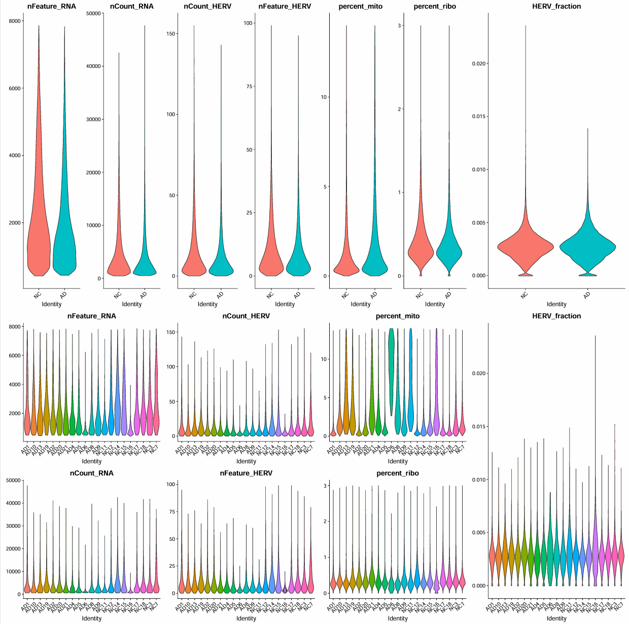
过滤前
library(Seurat)
library(tidyverse)
library(patchwork)
library(Matrix)
seu <- readRDS("/public/home/GENE_proc/wth/GSE157827/my_data/GSE157827.rds")
res_dir <- "/public/home/GENE_proc/wth/GSE157827/res/"
feats <- c("nFeature_RNA", "nCount_RNA")
p_filt_b_1 <- VlnPlot(
  seu, features = feats,
  pt.size = 0,
  ncol = 2,
  group.by = "group"
) + NoLegend()
p_filt_b_2 <- VlnPlot(
  seu, features = feats,
  pt.size = 0,
  ncol = 1,
  group.by = "orig.ident"
) + NoLegend()
feats <- c("percent_mito", "percent_ribo")
p_filt_b_3 <- VlnPlot(
  seu, features = feats,
  pt.size = 0,
  ncol = 2,
  group.by = "group"
) + NoLegend()
p_filt_b_4 <- VlnPlot(
  seu, features = feats,
  pt.size = 0,
  ncol = 1,
  group.by = "orig.ident"
) + NoLegend()
pdf(file.path(res_dir, "before_filter.pdf"))
p <- (p_filt_b_1 / p_filt_b_2) | (p_filt_b_3 / p_filt_b_4)
print(p)
dev.off()
> fivenum(seu@meta.data$nFeature_RNA)
[1]    38   948  1618  2783 14543
> fivenum(seu@meta.data$nCount_RNA)
[1]    450   1367   2697   5627 118970
> fivenum(seu@meta.data$nCount_HERV)
[1]   0   3   8  16 375
> fivenum(seu@meta.data$nFeature_HERV)
[1]   0   3   6  13 191
> fivenum(seu@meta.data$HERV_fraction)
[1] 0.000000000 0.001904762 0.002690704 0.003473227 0.022727273
> fivenum(seu@meta.data$percent_mito)
[1]  0.0000000  0.4662729  1.0680017  2.6499303 96.6913580
> fivenum(seu@meta.data$percent_ribo)
[1]  0.0000000  0.2367424  0.3400397  0.5042546 15.1050420
设置阈值
# 细胞阈值
retained_c_umi_low <- seu$nFeature_RNA > 500
retained_c_umi_high <- seu$nFeature_RNA < 8000
retained_c_count_low  <- seu$nCount_RNA > 1000
retained_c_count_high <- seu$nCount_RNA < 40000
retained_c_mito <- seu$percent_mito < 14
retained_c_ribo <- seu$percent_ribo < 3
keep_cells <- retained_c_mito & retained_c_ribo & retained_c_umi_low & retained_c_umi_high
scRNA_cells <- subset(seu, cells = Cells(seu)[keep_cells])
counts_rna <- GetAssayData(scRNA_cells, assay = "RNA", slot = "counts")
feature_rowsum <- Matrix::rowSums(counts_rna > 0)
# 基因阈值
retained_f_low <- feature_rowsum > ncol(scRNA_cells) * 0.005
genes_keep <- names(feature_rowsum)[retained_f_low]
counts_herv <- GetAssayData(scRNA_cells, assay = "HERV", slot = "counts")
herv_rowsum <- Matrix::rowSums(counts_herv > 0)
# hERV位点阈值
herv_cutoff <- ceiling(ncol(scRNA_cells) * 0.0001)
herv_keep <- names(herv_rowsum)[herv_rowsum > herv_cutoff]
cat("HERV features before:", nrow(counts_herv), "\n")  # 14969
cat("HERV features kept:", length(herv_keep), "\n")  # 4326
过滤
scRNA_cells[["RNA"]] <- subset(scRNA_cells[["RNA"]], features = genes_keep)
scRNA_cells[["HERV"]] <- subset(scRNA_cells[["HERV"]], features = herv_keep)
scRNA_cells
table(scRNA_cells$group)
table(scRNA_cells$orig.ident)
rna_counts <- GetAssayData(scRNA_cells, assay = "RNA", slot = "counts")
scRNA_cells$nCount_RNA <- Matrix::colSums(rna_counts)
scRNA_cells$nFeature_RNA <- Matrix::colSums(rna_counts > 0)
herv_counts <- GetAssayData(scRNA_cells, assay = "HERV", slot = "counts")
scRNA_cells$nCount_HERV <- Matrix::colSums(herv_counts)
scRNA_cells$nFeature_HERV <- Matrix::colSums(herv_counts > 0)
scRNA_cells$HERV_fraction <- scRNA_cells$nCount_HERV / (scRNA_cells$nCount_HERV + scRNA_cells$nCount_RNA)
过滤后结果
feats <- c("nFeature_RNA", "nCount_RNA")
p_filt_a_1 <- VlnPlot(
  scRNA_cells, features = feats,
  pt.size = 0,
  ncol = 2,
  group.by = "group"
) + NoLegend()
p_filt_a_2 <- VlnPlot(
  scRNA_cells, features = feats,
  pt.size = 0,
  ncol = 1,
  group.by = "orig.ident"
) + NoLegend()
# HERV?
feats <- c("nCount_HERV", "nFeature_HERV")
p_filt_a_3 <- VlnPlot(
  scRNA_cells, features = feats,
  pt.size = 0,
  ncol = 2,
  group.by = "group"
) + NoLegend()
p_filt_a_4 <- VlnPlot(
  scRNA_cells, features = feats,
  pt.size = 0,
  ncol = 1,
  group.by = "orig.ident"
) + NoLegend()
p_filt_a_7 <- VlnPlot(
  scRNA_cells, features = "HERV_fraction",
  pt.size = 0,
  ncol = 1,
  group.by = "group"
) + NoLegend()
p_filt_a_8 <- VlnPlot(
  scRNA_cells, features = "HERV_fraction",
  pt.size = 0,
  ncol = 1,
  group.by = "orig.ident"
) + NoLegend()
feats <- c("percent_mito", "percent_ribo")
p_filt_a_5 <- VlnPlot(
  scRNA_cells, features = feats,
  pt.size = 0,
  ncol = 2,
  group.by = "group"
) + NoLegend()
p_filt_a_6 <- VlnPlot(
  scRNA_cells, features = feats,
  pt.size = 0,
  ncol = 1,
  group.by = "orig.ident"
) + NoLegend()
pdf(file.path(res_dir, "after_filter.pdf"), width = 20, height = 20)
p <- (p_filt_a_1 / p_filt_a_2) | (p_filt_a_3 / p_filt_a_4) | (p_filt_a_5 / p_filt_a_6) | (p_filt_a_7 / p_filt_a_8)
print(p)
dev.off()
# 保存数据
saveRDS(
    scRNA_cells,
    file = "/public/home/GENE_proc/wth/GSE157827/my_data/GSE157827_filt.rds",
    compress = "xz"
)
最终结果:
> dim(scRNA_cells)  # 不包括hERV
[1]  21002 164219
> table(scRNA_cells$GSM)
GSM4775561 GSM4775562 GSM4775563 GSM4775564 GSM4775565 GSM4775566 GSM4775567 GSM4775568 GSM4775569
      5865      15080       5435      12140        230       2167       9238      15703       1517
GSM4775570 GSM4775571 GSM4775572 GSM4775573 GSM4775574 GSM4775575 GSM4775576 GSM4775577 GSM4775578
      3549       9037       7691       6056       6130       1520      15185      10596       8175
GSM4775579 GSM4775580 GSM4775581
      3554      13900      11451
作者的计数矩阵过滤后:
> dim(scRNA_filt)
[1]  17276 169516
> table(scRNA_filt$orig.ident)
GSM4775561 GSM4775562 GSM4775563 GSM4775564 GSM4775565 GSM4775566 GSM4775567 GSM4775568 GSM4775569
      6173      15276       5980      12356        311       2405       9789      16013       1608
GSM4775570 GSM4775571 GSM4775572 GSM4775573 GSM4775574 GSM4775575 GSM4775576 GSM4775577 GSM4775578
      3614       9169       7786       6218       6372       1587      15568      10932       8385
GSM4775579 GSM4775580 GSM4775581
      4235      14263      11476
与作者的计数矩阵对照
library(Seurat)
library(tidyverse)
library(patchwork)
library(Matrix)
seu_auth <- readRDS("/public/home/GENE_proc/wth/GSE157827/raw_data/GSE157827_filt.rds")
seu_ours <- readRDS("/public/home/GENE_proc/wth/GSE157827/my_data/GSE157827_filt.rds")
res_dir <- "/public/home/GENE_proc/wth/GSE157827/res/"
auth_cells <- colnames(seu_auth)
our_cells <- colnames(seu_ours)
common_cells <- intersect(auth_cells, our_cells)
mat_ours <- GetAssayData(seu_ours, assay = "RNA", slot = "counts")
mat_auth <- GetAssayData(seu_auth, assay = "RNA", slot = "counts")
common_genes <- intersect(rownames(mat_ours), rownames(mat_auth))
> cat("ours cells:", length(our_cells), "\n")
ours cells: 164219
> cat("auth cells:", length(auth_cells), "\n")
auth cells: 169516
> cat("common cells:", length(common_cells), "\n")
common cells: 161921
> cat("overlap % (of ours):", round(length(common_cells)/length(our_cells)*100, 2), "%\n")
overlap % (of ours): 98.6 %
> cat("overlap % (of auth):", round(length(common_cells)/length(auth_cells)*100, 2), "%\n")
overlap % (of auth): 95.52 %
> cat("ours genes:", length(rownames(mat_ours)), "\n")
ours genes: 21002
> cat("auth genes:", length(rownames(mat_auth)), "\n")
auth genes: 17276
> cat("common genes:", length(common_genes), "\n")
common genes: 13938
> cat("overlap % (of ours):", round(length(common_genes)/length(rownames(mat_ours))*100, 2), "%\n")
overlap % (of ours): 66.37 %
> cat("overlap % (of auth):", round(length(common_genes)/length(rownames(mat_auth))*100, 2), "%\n")
overlap % (of auth): 80.68 %
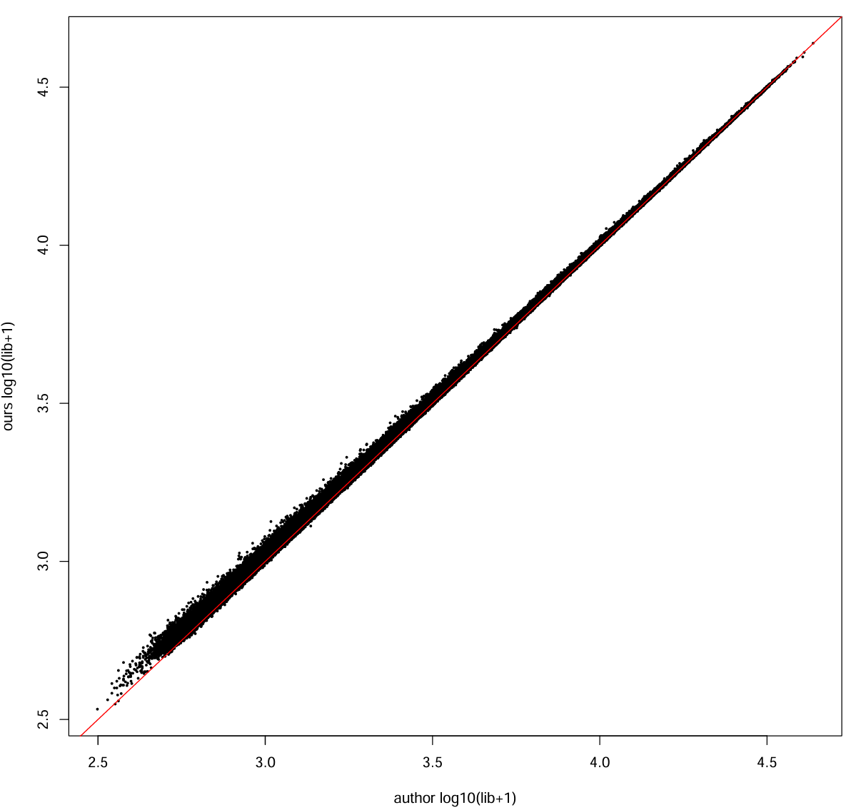
在重叠的细胞上比较计数的一致性:
每个细胞的总UMI:
mat_ours_sub <- mat_ours[common_genes, common_cells, drop = FALSE]
mat_auth_sub <- mat_auth[common_genes, common_cells, drop = FALSE]
our_lib  <- Matrix::colSums(mat_ours_sub)
auth_lib <- Matrix::colSums(mat_auth_sub)
cor_lib <- cor(log10(our_lib + 1), log10(auth_lib + 1))
cat("cell library size corr (log10+1):", cor_lib, "\n")  # 0.9997134
pdf(file.path(res_dir, "author_our_umi.pdf"), width = 10, height = 10)
plot(log10(auth_lib + 1), log10(our_lib + 1),
     xlab = "author log10(lib+1)", ylab = "ours log10(lib+1)", pch = 16, cex = 0.4)
abline(0, 1, col = "red")
dev.off()
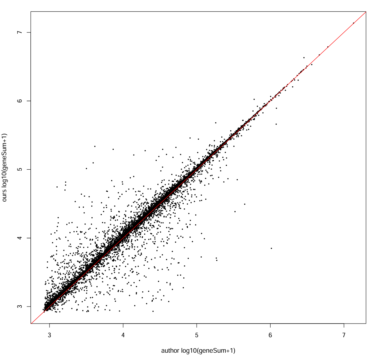
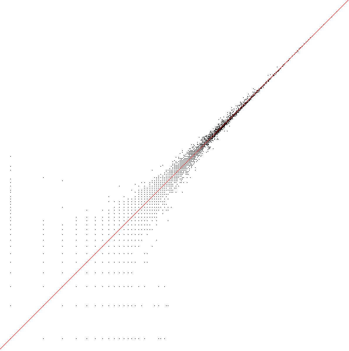
每个基因的总counts:
our_gene_sum  <- Matrix::rowSums(mat_ours_sub)
auth_gene_sum <- Matrix::rowSums(mat_auth_sub)
cor_gene <- cor(log10(our_gene_sum + 1), log10(auth_gene_sum + 1))
cat("gene total counts corr (log10+1):", cor_gene, "\n")  # 0.9746644
pdf(file.path(res_dir, "author_our_counts.pdf"), width = 10, height = 10)
plot(log10(auth_gene_sum + 1), log10(our_gene_sum + 1),
     xlab = "author log10(geneSum+1)", ylab = "ours log10(geneSum+1)", pch = 16, cex = 0.4)
abline(0, 1, col = "red")
dev.off()
每个细胞的基因向量相关性(随机抽3k细胞×3k基因):
set.seed(1)
v_my <- as.vector(log1p(mat_ours_sub))
v_auth <- as.vector(log1p(mat_auth_sub))
cells_sample <- sample(colnames(mat_ours_sub), 3000)
genes_sample <- sample(rownames(mat_ours_sub), 3000)
my_sub <- as.matrix(mat_ours_sub[genes_sample, cells_sample])
auth_sub <- as.matrix(mat_auth_sub[genes_sample, cells_sample])
v_my_sub <- as.vector(log1p(my_sub))
v_auth_sub <- as.vector(log1p(auth_sub))
cor_flat <- cor(v_my_sub, v_auth_sub)
cor_flat  # 0.9677604
pdf(file.path(res_dir, "author_our_corr.pdf"), width = 10, height = 10)
par(pin = c(10, 10))
plot(v_my_sub, v_auth_sub, pch = ".", xlab = "log1p(my)", ylab = "log1p(author)")
abline(0, 1, col = "red")
dev.off()
抽取一部分细胞到本地
scRNA_cells <- readRDS("/public/home/GENE_proc/wth/GSE157827/my_data/GSE157827_filt.rds")
set.seed(20260102)
prop_keep <- 1/3
cells_keep <- scRNA_cells@meta.data %>%
  rownames_to_column("cell") %>%
  group_by(orig.ident) %>%
  slice_sample(prop = prop_keep) %>%
  pull(cell)
scRNA_smaller <- subset(scRNA_cells, cells = cells_keep)
saveRDS(
    scRNA_smaller,
    file = "/public/home/GENE_proc/wth/GSE157827/my_data/GSE157827_filt_smaller.rds",
    compress = "xz"
)
> ncol(scRNA_smaller)
[1] 54731
> table(scRNA_smaller$group)
   NC    AD
25519 29212
> table(scRNA_smaller$orig.ident)
 AD1 AD10 AD13 AD19  AD2 AD20 AD21  AD4  AD5  AD6  AD8  AD9 NC11 NC12 NC14 NC15 NC16 NC17 NC18  NC3
1955 5234  505 1183 5026 3012 2563 1811 4046   76  722 3079  506 5061 3532 2725 1184 4633 3817 2018
 NC7
2043
数据预处理
library(Seurat)
library(tidyverse)
library(patchwork)
library(Matrix)
library(clustree)
# seu <- readRDS("C:\\Users\\17185\\Desktop\\hERV_calc\\GSE157827\\my_data\\GSE157827_filt_smaller.rds")
# res_dir <- "C:\\Users\\17185\\Desktop\\hERV_calc\\GSE157827\\my_res"
seu <- readRDS("/public/home/GENE_proc/wth/GSE157827/my_data/GSE157827_filt.rds")
res_dir <- "/public/home/GENE_proc/wth/GSE157827/res/"
RNA:常规预处理
seu <- NormalizeData(
seu,
assay = "RNA",
normalization.method = "LogNormalize",
scale.factor = 10000
)
seu <- FindVariableFeatures(
seu,
assay = "RNA",
selection.method = "vst",
nfeatures = 2000
)
seu <- ScaleData(
seu,
assay = "RNA",
features = VariableFeatures(seu),
vars.to.regress = c("nFeature_RNA", "percent_mito")
)
seu <- RunPCA(
seu,
assay = "RNA",
features = VariableFeatures(seu),
npcs = 50
)
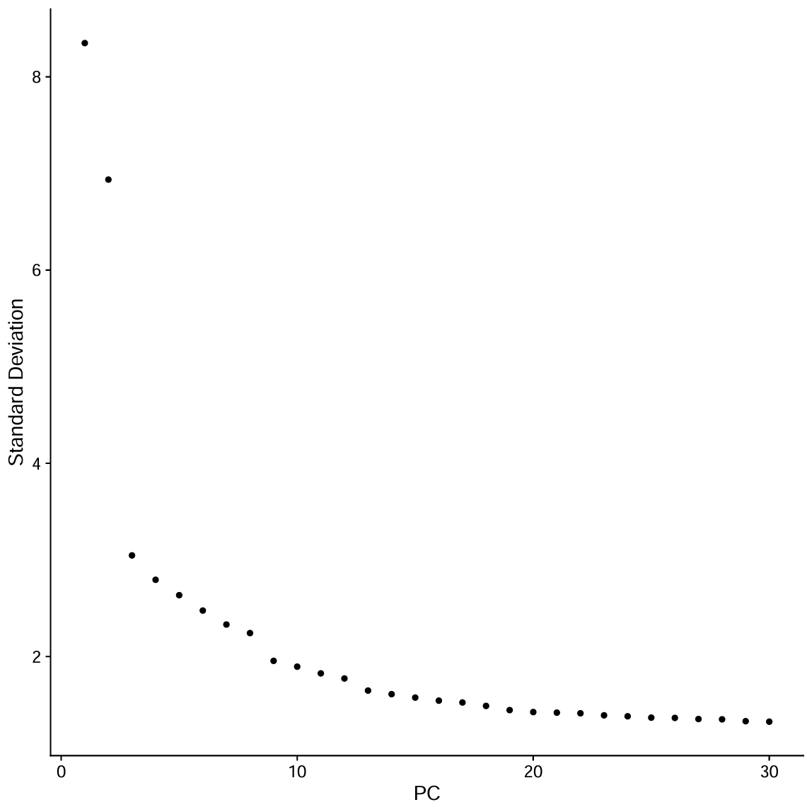
pdf(file.path(res_dir, "ElbowPlot_all.pdf"))
p <- ElbowPlot(seu, ndims = 50, reduction = "pca")
print(p)
dev.off()
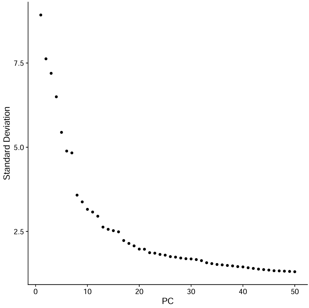
pc.use <- 1:30
seu <- RunUMAP(seu, reduction = "pca", dims = pc.use)
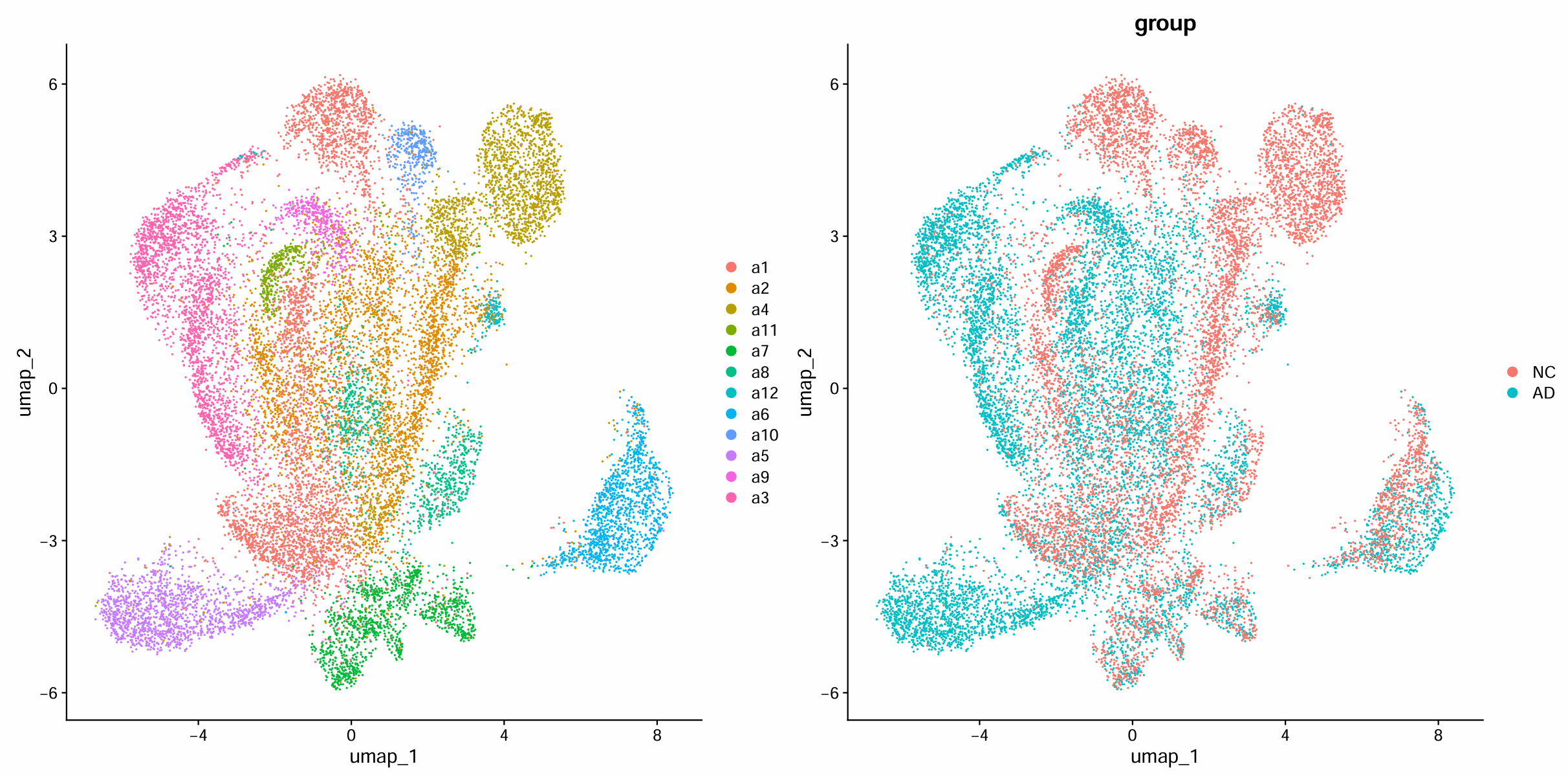
p_dim_group <- DimPlot(seu, group.by = "group")
p_dim_gsm <- DimPlot(seu, group.by = "orig.ident", raster = TRUE)
seu <- FindNeighbors(seu, dims = pc.use)
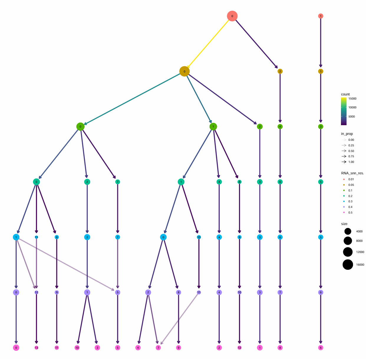
seu <- FindClusters(seu, resolution = c(0.01, 0.05, 0.1, 0.2, 0.5))
p_cutree <- clustree(seu@meta.data, prefix = "RNA_snn_res.")
# 选一个resolution作为最终cluster标签(教程选0.05)
Idents(seu) <- seu$RNA_snn_res.0.05
# 把cluster编号标到UMAP上
p_dim_cluster <- DimPlot(seu, label = TRUE)
# 拼图展示
pdf(file.path(res_dir, "data_preprocess.pdf"), width = 16, height = 16)
p <- (p_dim_group | p_dim_gsm) / (p_cutree | p_dim_cluster)
print(p)
dev.off()
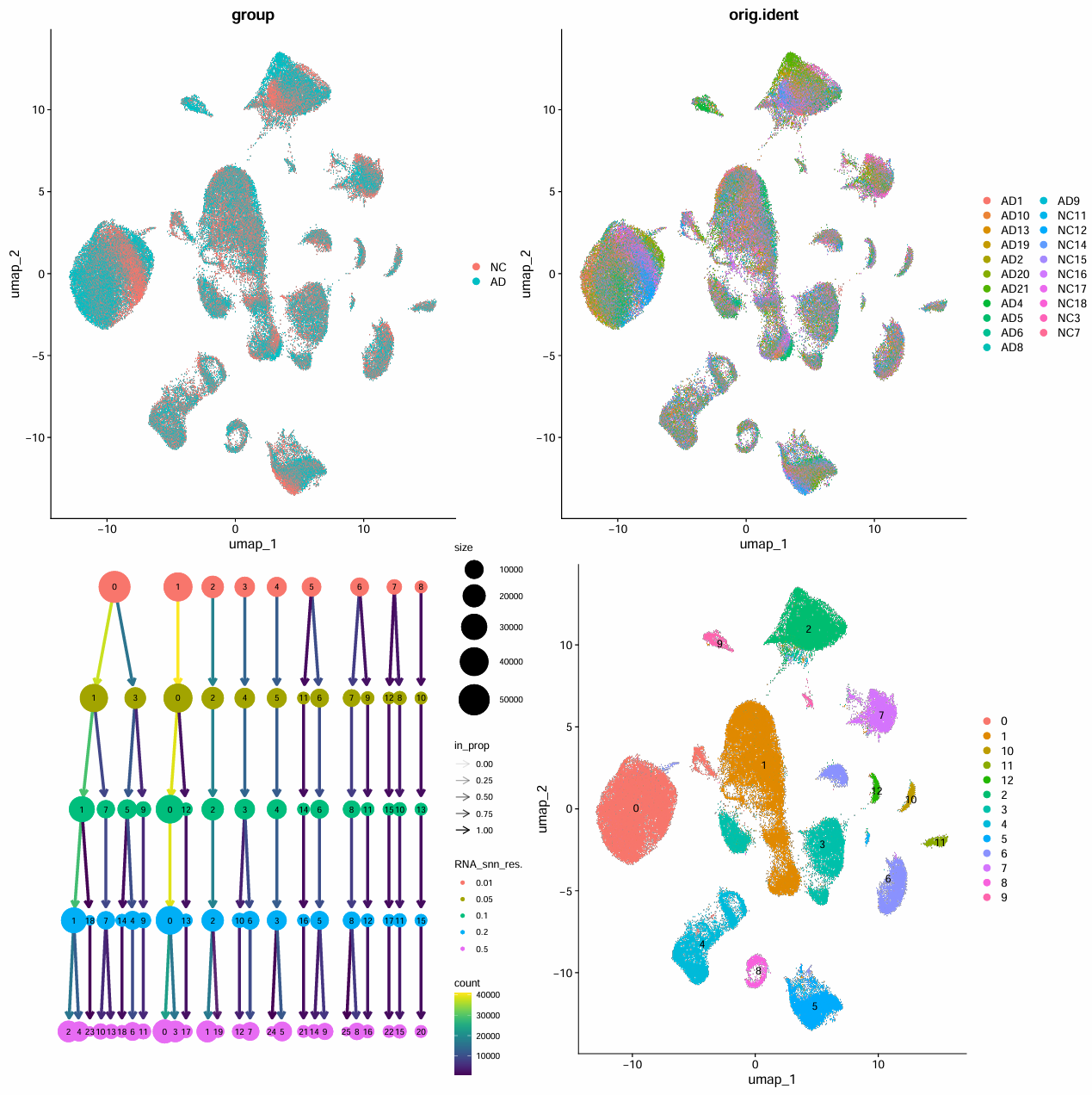
按样本混合的较均匀,目前不需要去批次效应
HERV:特殊方法
用RNA的库深度(nCount_RNA)做LogNormalize
normalize_herv_by_rna_depth <- function(seu, scale.factor = 10000) {
  rna_counts  <- GetAssayData(seu, assay = "RNA",  slot = "counts")
  herv_counts <- GetAssayData(seu, assay = "HERV", slot = "counts")
  lib_rna <- Matrix::colSums(rna_counts)  # 基因counts作size factor
  herv_norm <- t(t(herv_counts) / lib_rna) * scale.factor
  herv_norm@x <- log1p(herv_norm@x)
  seu <- SetAssayData(seu, assay = "HERV", slot = "data", new.data = herv_norm)
  seu$HERV_fraction <- seu$nCount_HERV / (seu$nCount_HERV + seu$nCount_RNA)
  return(seu)
}
DefaultAssay(seu) <- "HERV"
seu <- normalize_herv_by_rna_depth(seu, scale.factor = 10000)
检查标准化结果是否正确
get_mat <- function(seu, assay, slot) {
tryCatch(
GetAssayData(seu, assay = assay, slot = slot),
error = function(e) LayerData(seu, assay = assay, layer = slot)
)
}
rna_counts <- get_mat(seu, "RNA", "counts")
herv_counts <- get_mat(seu, "HERV", "counts")
herv_data <- get_mat(seu, "HERV", "data")
# RNA库深度一致性
rna_lib <- Matrix::colSums(rna_counts)
cat("cor(meta nCount_RNA, colSums(RNA counts)) = ",
cor(seu$nCount_RNA, rna_lib), "\n")
print(summary(seu$nCount_RNA - as.numeric(rna_lib)))
# 验证计算正确性
set.seed(1)
cells <- sample(colnames(seu), 200)
feats <- sample(rownames(herv_counts), min(200, nrow(herv_counts)))
hsub <- herv_counts[feats, cells, drop = FALSE]
rna_lib_sub <- as.numeric(rna_lib[cells])
manual <- log1p(t(t(as.matrix(hsub)) / rna_lib_sub * 10000))
stored <- as.matrix(herv_data[feats, cells, drop = FALSE])
cat("max(abs(manual - stored)) = ", max(abs(manual - stored)), "\n")
cat("cor(manual, stored) = ", cor(as.vector(manual), as.vector(stored)), "\n")
# HERV_fraction一致性
herv_lib <- Matrix::colSums(herv_counts)
frac_manual <- as.numeric(herv_lib) / (as.numeric(rna_lib) + as.numeric(herv_lib))
cat("cor(meta HERV_fraction, manual) = ", cor(seu$HERV_fraction, frac_manual), "\n")
print(summary(seu$HERV_fraction - frac_manual))
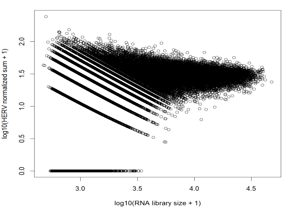
# 标准化后是否仍强依赖RNA库深度
# HERV线性归一化总量(未log)与RNA库深度(应明显减弱相关)
herv_norm_linear <- as.numeric(herv_lib) / as.numeric(rna_lib) * 10000
plot(log10(as.numeric(rna_lib) + 1), log10(herv_norm_linear + 1),
xlab = "log10(RNA library size + 1)",
ylab = "log10(HERV normalized sum + 1)")
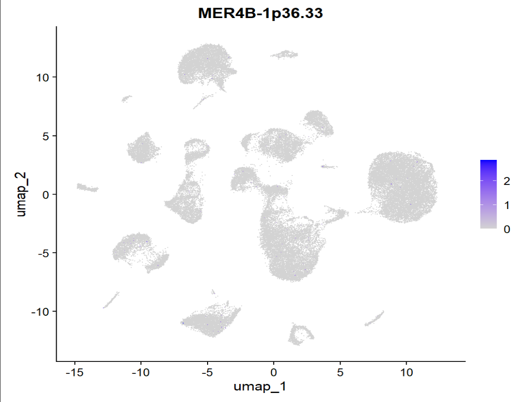
# 随便挑一个HERV feature(你也可以换成你感兴趣的ERV位点)看FeaturePlot
DefaultAssay(seu) <- "HERV"
feat1 <- rownames(herv_counts)[3]
FeaturePlot(seu, features = feat1, reduction = "umap")
> cat("cor(meta nCount_RNA, colSums(RNA counts)) = ", cor(seu$nCount_RNA, rna_lib), "\n")
cor(meta nCount_RNA, colSums(RNA counts)) =  1
> print(summary(seu$nCount_RNA - as.numeric(rna_lib)))
   Min. 1st Qu.  Median    Mean 3rd Qu.  Max.
      0       0       0       0       0    0
> cat("max(abs(manual - stored)) = ", max(abs(manual - stored)), "\n")
max(abs(manual - stored)) =  0
> cat("cor(manual, stored) = ", cor(as.vector(manual), as.vector(stored)), "\n")
cor(manual, stored) =  1
> cat("cor(meta HERV_fraction, manual) = ", cor(seu$HERV_fraction, frac_manual), "\n")
cor(meta HERV_fraction, manual) =  1
> print(summary(seu$HERV_fraction - frac_manual))
   Min. 1st Qu.  Median    Mean 3rd Qu.    Max.
      0       0       0       0       0       0
标准化结果是合理的
- 对于第一张图,随着RNA_lib增大,hERV总counts会按1/RNA_lib下降,因此出现成排斜线(每条线对应一个固定的系数);同时低RNA库深度的细胞上hERV方差更大,因此左侧更散
- 对于第二张图,每细胞HERV总量≈8、RNA_lib≈2700,标准化后范围大概在1.3~1.7
- 大部分hERV位点在大部分细胞里计数为0
- 标准化后,非0的值通常在0~3左右
细胞注释
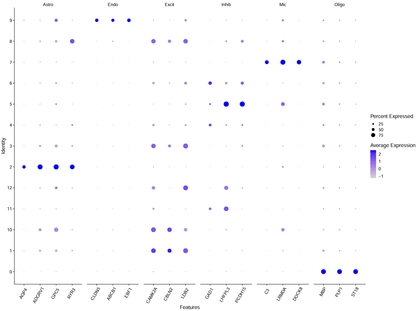
DefaultAssay(seu) <- "RNA"
# marker基因
gene_list <- list(
  Astro = c("AQP4", "ADGRV1", "GPC5", "RYR3"),
  Endo  = c("CLDN5", "ABCB1", "EBF1"),
  Excit = c("CAMK2A", "CBLN2", "LDB2"),
  Inhib = c("GAD1", "LHFPL3", "PCDH15"),
  Mic   = c("C3", "LRMDA", "DOCK8"),
  Oligo = c("MBP", "PLP1", "ST18")
)
# 在各个聚类中的表达量
pdf(file.path(res_dir, "cluster_marker_gene.pdf"), width = 16, height = 12)
p <- DotPlot(seu, features = gene_list, assay = "RNA") +
  theme(axis.text.x = element_text(angle = 60, vjust = 0.8, hjust = 0.8))
print(p)
dev.off()
# 计算每个cluster对每个细胞类型的marker-set的平均表达
score_by_cluster <- function(seu, gene_list, group_col) {
  out <- lapply(names(gene_list), function(ct) {
    feats <- intersect(gene_list[[ct]], rownames(seu))
    if (length(feats) == 0) return(NULL)
    avg <- AverageExpression(
      seu,
      assays = "RNA",
      features = feats,
      group.by = group_col,
      slot = "data",
      verbose = FALSE
    )$RNA  # features x clusters
    data.frame(
      cluster = colnames(avg),
      celltype = ct,
      score = colMeans(avg, na.rm = TRUE),
      stringsAsFactors = FALSE
    )
  }) |> bind_rows()
  tab <- out |>
    pivot_wider(names_from = celltype, values_from = score) |>
    arrange(as.numeric(as.character(cluster)))
  mat <- as.matrix(tab[, intersect(names(gene_list), colnames(tab)), drop = FALSE])
  tab$pred <- colnames(mat)[max.col(mat, ties.method = "first")]
  tab
}
score_tab <- score_by_cluster(seu, gene_list, "RNA_snn_res.0.05")
print(score_tab, n = nrow(score_tab))
抽样数据:
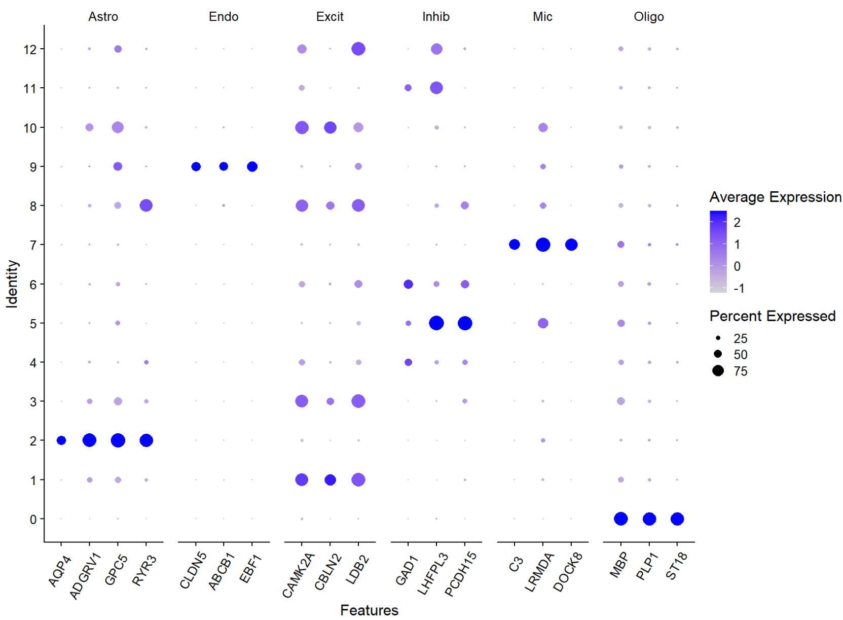
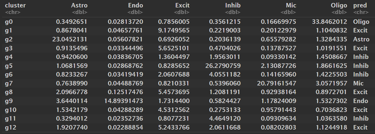
- Oligodendrocyte:0
- Astrocyte:2
- Microglia:7
- Endothelial:9
- Inhibitory neuron:4、5、6、11
- Excitatory neuron:1、3、8、10、12
全部数据:
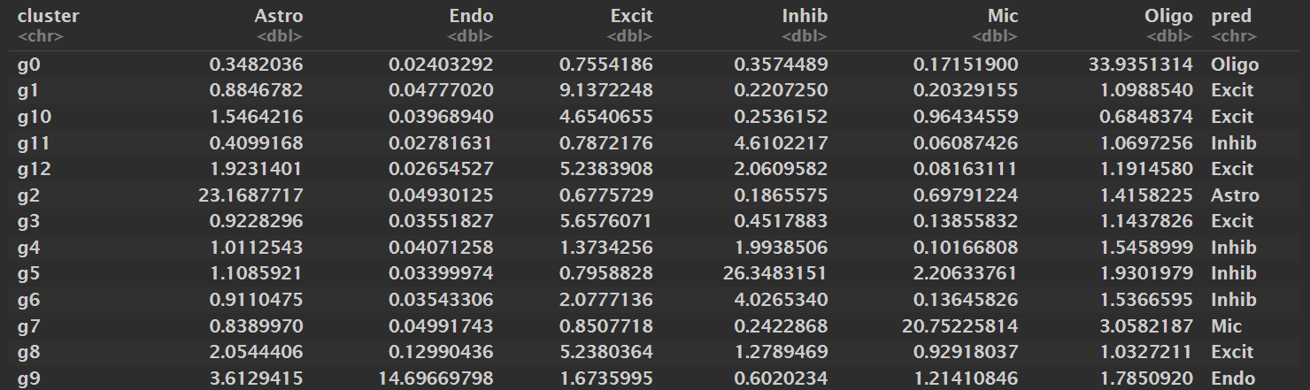
很巧合的,全部数据的聚类结果和抽样数据的完全相同
cl_Astro <- c("2")
cl_Endo  <- c("9")
cl_Mic   <- c("7")
cl_Oligo <- c("0")
cl_Inhib <- c("4", "5", "6", "11")
# 其它细胞归为Excit
cl <- as.character(seu[["RNA_snn_res.0.05"]][, 1])
seu$celltype <- ifelse(cl %in% cl_Astro, "Astro",
                  ifelse(cl %in% cl_Endo,  "Endo",
                    ifelse(cl %in% cl_Mic,   "Mic",
                      ifelse(cl %in% cl_Oligo, "Oligo",
                        ifelse(cl %in% cl_Inhib, "Inhib", "Excit")))))
seu$celltype <- factor(seu$celltype, levels = c("Astro","Endo","Excit","Inhib","Mic","Oligo"))
Idents(seu) <- seu$celltype
table(seu$celltype, seu$group)
# 保存数据
saveRDS(
    seu,
    # file = "C:\\Users\\17185\\Desktop\\hERV_calc\\GSE157827\\my_data\\GSE157827_smaller_celltype.rds",
    file = "C:\\Users\\17185\\Desktop\\hERV_calc\\GSE157827\\my_data\\GSE157827_celltype.rds",
    compress = "xz"
)
> table(seu$celltype, seu$group)
           NC    AD
  Astro  8411  9695
  Endo    566  1589
  Excit 28234 31031
  Inhib 17585 18747
  Mic    3555  3909
  Oligo 18216 22681
> table(seu$celltype)
Astro  Endo Excit Inhib   Mic Oligo
18106  2155 59265 36332  7464 40897
教程里的注释:
> table(scRNA$celltype, useNA = "ifany")
Astro  Endo Excit Inhib   Mic Oligo
19120  2241 62093 37239  7773 41050
基本没有差别
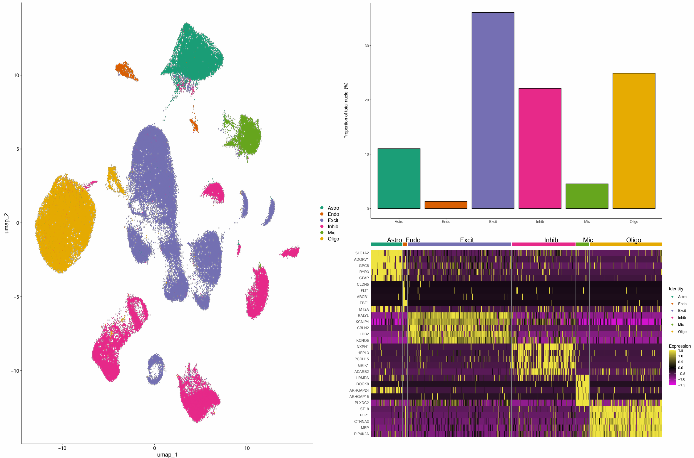
画图展示
ct_cols <- c(
  Astro = "#1b9e77",
  Endo  = "#d95f02",
  Excit = "#7570b3",
  Inhib = "#e7298a",
  Mic   = "#66a61e",
  Oligo = "#e6ab02"
)
# 细胞类型在umap上的分布
dim_plot <- DimPlot(
  seu,
  reduction = "umap",
  cols = ct_cols,
  label = FALSE
)
# 统计各细胞类型的细胞数和比例
ct_stat <- as.data.frame(table(seu$celltype))
colnames(ct_stat) <- c("celltype", "total")
ct_stat$celltype <- factor(ct_stat$celltype, levels = levels(seu@active.ident))
ct_stat$percentage <- 100 * ct_stat$total / sum(ct_stat$total)
celltype_bar <- ggplot(ct_stat, aes(x = celltype, y = percentage, fill = celltype)) +
  geom_bar(stat = "identity", color = "black") +
  scale_fill_manual(values = ct_cols) +
  theme_classic() +
  theme(axis.title.x = element_blank(), legend.position = "none") +
  ylab("Proportion of total nuclei (%)")
# 各细胞类型marker热图
genes_paper <- c(
  "SLC1A2","ADGRV1","GPC5","RYR3","GFAP",
  "CLDN5","FLT1","ABCB1","EBF1","MT2A",
  "RALYL","KCNIP4","CBLN2","LDB2","KCNQ5",
  "NXPH1","LHFPL3","PCDH15","GRIK1","ADARB2",
  "LRMDA","DOCK8","ARHGAP24","ARHGAP15","PLXDC2",
  "ST18","PLP1","CTNNA3","MBP","PIP4K2A"
)
genes_use <- intersect(genes_paper, rownames(seu))
length(genes_use) == length(genes_paper)  # 全在我的数据集中
seu <- ScaleData(seu, features = genes_use, verbose = FALSE)
heatmap <- DoHeatmap(
  seu,
  features = genes_use,
  disp.min = -1.5,
  disp.max = 1.5,
  angle = 0,
  group.colors = unname(ct_cols)
) + scale_fill_gradientn(
  colors = c("#f100ef", "black", "#f0e442"),
  limits = c(-1.5, 1.5)
)
pdf(file.path(res_dir, "celltype.pdf"), width = 24, height = 16)
p <- dim_plot + celltype_bar / heatmap
print(p)
dev.off()
计算差异基因,便于后面计算富集分数
scRNA <- readRDS("/public/home/GENE_proc/wth/GSE157827/my_data/GSE157827_celltype.rds")
DefaultAssay(scRNA) <- "RNA"
scRNA$group <- factor(scRNA$group, levels = c("NC","AD"))
scRNA$celltype <- factor(
  scRNA$celltype,
  levels = c("Astro","Endo","Excit","Inhib","Mic","Oligo")
)
Idents(scRNA) <- scRNA$celltype
balance_cells <- function(obj, ct){
  sub <- subset(obj, idents = ct)
  ad <- WhichCells(sub, expression = group == "AD")
  nc <- WhichCells(sub, expression = group == "NC")
  if(length(ad) > 2000){
    n <- min(length(ad), length(nc))
    sub[, c(sample(ad, n), sample(nc, n))]
  } else {
    sub
  }
}
cts <- levels(scRNA$celltype)
obj_bal <- merge(x = balance_cells(scRNA, cts[1]),
                 y = lapply(cts[-1], \(ct) balance_cells(scRNA, ct)))
obj_bal$celltype <- factor(
  obj_bal$celltype,
  levels = c("Astro","Endo","Excit","Inhib","Mic","Oligo")
)
obj_bal <- JoinLayers(obj_bal, assay = "RNA")
obj_bal$compare <- paste(obj_bal$group, obj_bal$celltype, sep = "_")
scRNA$compare <- paste(scRNA$group, scRNA$celltype, sep = "_")
ct <- levels(obj_bal$celltype)
all_markers <- lapply(ct, function(x){
  message("Running: ", x)
  FindMarkers(
    obj_bal,
    group.by = "compare",
    ident.1 = paste0("AD_", x),
    ident.2 = paste0("NC_", x),
    logfc.threshold = 0.25,
    min.pct = 0.1
  )
})
names(all_markers) <- ct
lapply(all_markers, nrow)
all_markers_sig <- lapply(all_markers, function(df){
  df2 <- subset(
    df,
    p_val_adj < 0.1
  )
  return(df2)
})
View(all_markers_sig[["Astro"]])
save(all_markers_sig, file = "/public/home/GENE_proc/wth/GSE157827/my_data/GSE157827_all_markers_sig.RData")
差异表达分析
library(Seurat)
library(tidyverse)
library(patchwork)
library(Matrix)
library(clustree)
library(edgeR)
# seu <- readRDS("C:\\Users\\17185\\Desktop\\hERV_calc\\GSE157827\\my_data\\GSE157827_smaller_celltype.rds")
# res_dir <- "C:\\Users\\17185\\Desktop\\hERV_calc\\GSE157827\\my_res"
seu <- readRDS("/public/home/GENE_proc/wth/GSE157827/my_data/GSE157827_celltype.rds")
res_dir <- "/public/home/GENE_proc/wth/GSE157827/res/"
细胞类型level
根据开题报告里的大致思路,先尝试pseudo-bulk
sample_col <- "orig.ident"
seu$sample <- seu@meta.data[[sample_col]]
seu$group  <- factor(seu$group, levels = c("NC", "AD"))
# 每个细胞类型在AD/NC里各有多少个样本(该样本在该细胞类型下至少有1个细胞)
cell_n <- as.data.frame(table(celltype = seu$celltype, sample = seu$sample, group = seu$group)) %>%
  filter(Freq > 0)
sample_stat <- cell_n %>%
  group_by(celltype, group) %>%
  summarise(
    n_samples = n_distinct(sample),
    min_cells = min(Freq),
    median_cells = as.numeric(median(Freq)),
    .groups = "drop"
  ) %>%
  arrange(celltype, group)
# pseudo-bulk的计数矩阵(按细胞类型+样本聚合)
pb <- AggregateExpression(
  seu,
  assays = c("RNA", "HERV"),
  group.by = c("celltype", "sample"),
  slot = "counts",
  verbose = FALSE
)
pb_rna_counts  <- pb$RNA
pb_herv_counts <- pb$HERV
# 添加AD/NC信息
cn <- colnames(pb_herv_counts)
pb_meta <- tibble(pb_col = cn) %>%
  mutate(parts = strsplit(pb_col, "_")) %>%
  rowwise() %>%
  mutate(
    celltype = parts[[1]][1],
    sample   = parts[[2]][1]
  ) %>%
  ungroup()
sample2group <- seu@meta.data %>%
  distinct(sample, group)
pb_meta <- pb_meta %>%
  left_join(sample2group, by = "sample") %>%
  mutate(group = factor(group, levels = c("NC","AD")))
# 检查NA
print(table(is.na(pb_meta$group)))
print(table(pb_meta$celltype, pb_meta$group))
# 保存数据
saveRDS(
  list(pb_rna_counts = pb_rna_counts, pb_herv_counts = pb_herv_counts, sample_stat = sample_stat, pb_meta = pb_meta),
  file = "/public/home/GENE_proc/wth/GSE157827/my_data/pseudobulk_counts_by_celltype_sample.rds"
)
先在一个细胞类型上算hERV的差异,这里选用astro做test
# readRDS("/public/home/GENE_proc/wth/GSE157827/my_data/pseudobulk_counts_by_celltype_sample.rds")
data <- readRDS("C:\\Users\\17185\\Desktop\\hERV_calc\\GSE157827\\my_data\\pseudobulk_counts_by_celltype_sample.rds")
pb_rna_counts = data[["pb_rna_counts"]]; pb_herv_counts = data[["pb_herv_counts"]]; sample_stat = data[["sample_stat"]]; pb_meta = data[["pb_meta"]]; rm(data)
run_edger_one <- function(count_mat, pb_meta, celltype) {
  idx <- pb_meta$celltype == celltype
  meta <- pb_meta[idx, ]
  y <- DGEList(counts = count_mat[, idx, drop = FALSE])
  y$samples$group <- meta$group
  cat("features before filterByExpr:", nrow(y), "\n")
  keep <- filterByExpr(y, group = y$samples$group)
  y <- y[keep, , keep.lib.sizes = FALSE]
  cat("features after  filterByExpr:", nrow(y), "\n")
  y <- calcNormFactors(y)
  design <- model.matrix(~ group, data = y$samples)  # NC为基线
  y <- estimateDisp(y, design)
  fit <- glmQLFit(y, design)
  qlf <- glmQLFTest(fit, coef = "groupAD")
  res <- topTags(qlf, n = Inf)$table
  res$feature <- rownames(res)
  rownames(res) <- NULL
  res
}
res_herv_astro <- run_edger_one(pb_herv_counts, pb_meta, "Astro")
View(res_herv_astro)
features before filterByExpr: 4326
features after  filterByExpr: 92
不是“多重校正把信号掩盖了(92不算多),而是信号本身就不够强,即pseudo-bulk在astro大类的hERV差异上不显著(不等于“完全没差异”,只是在现在的方法下达不到显著)
之后我尝试了普通单细胞的方法(FindMarkers)
astro <- subset(seu, subset = celltype == "Astro")
DefaultAssay(astro) <- "HERV"
Idents(astro) <- astro$group  # AD vs NC
sc_herv_astro <- FindMarkers(
  astro,
  ident.1 = "AD",
  ident.2 = "NC",
  assay = "HERV",
  slot = "data",
  test.use = "MAST",
  latent.vars = c("orig.ident")  # 把样本作为协变量,减轻伪重复
)
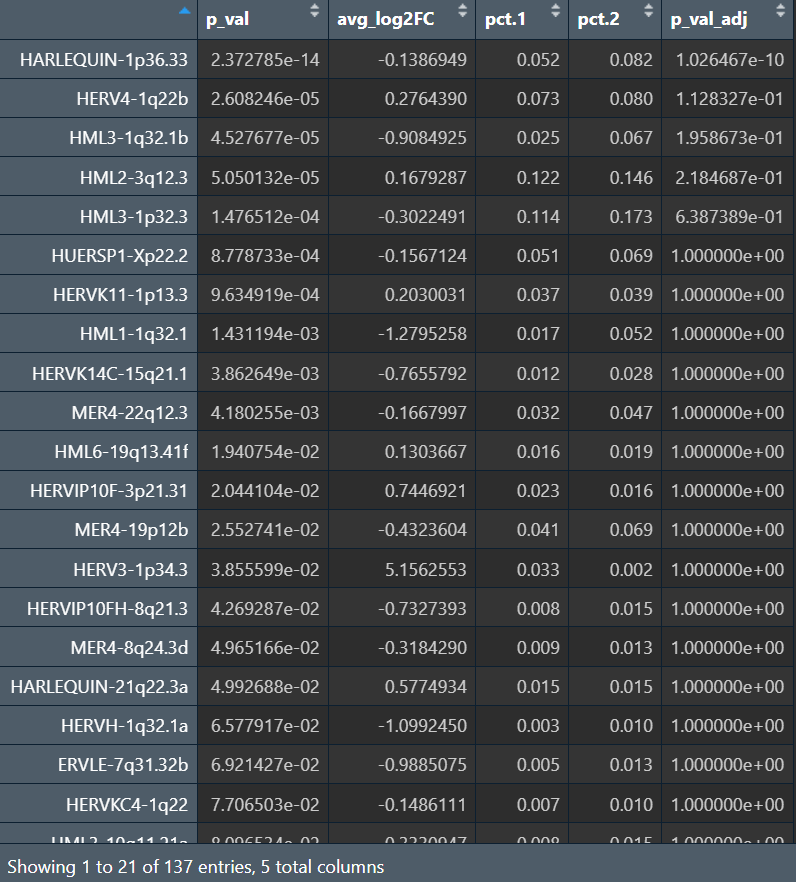
去掉latent.vars = c("orig.ident")后
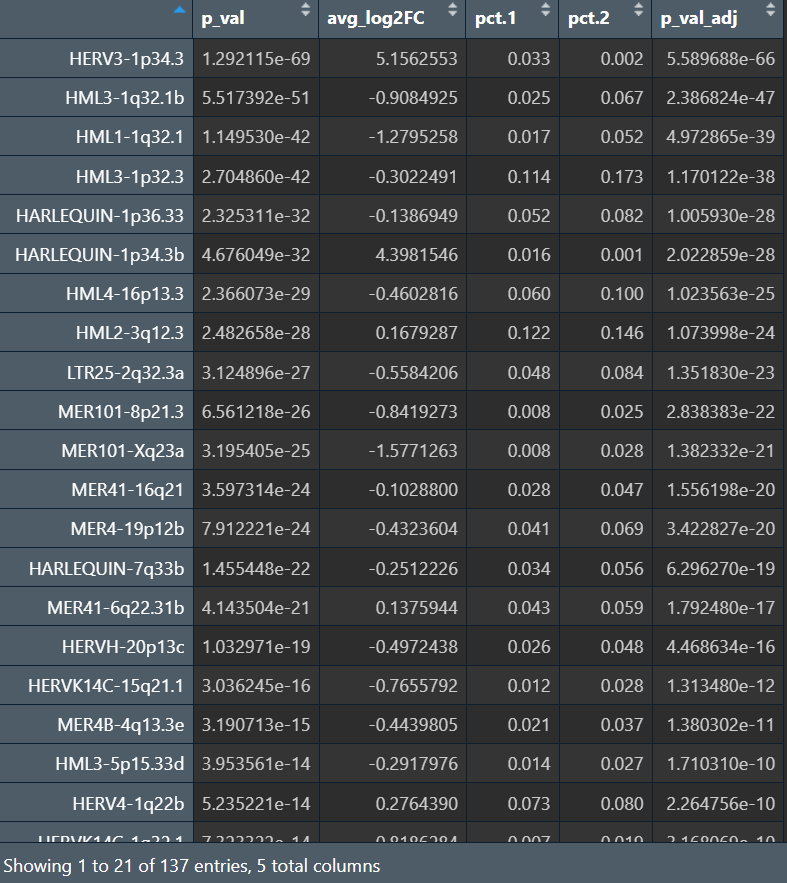
结果和pseudo-bulk也类似——把“样本/个体”作为协变量后,也只有少数能保持差异
对所有细胞类型都运行一遍pseudo-bulk分析流程
run_edger_one2 <- function(count_mat, pb_meta, celltype) {
idx <- pb_meta$celltype == celltype
meta <- pb_meta[idx, ]
y <- DGEList(counts = count_mat[, idx, drop = FALSE])
y$samples$group <- meta$group
n_before <- nrow(y)
keep <- filterByExpr(y, group = y$samples$group)
y <- y[keep, , keep.lib.sizes = FALSE]
n_after <- nrow(y)
y <- calcNormFactors(y)
design <- model.matrix(~ group, data = y$samples)
y <- estimateDisp(y, design)
fit <- glmQLFit(y, design)
qlf <- glmQLFTest(fit, coef = "groupAD")
res <- topTags(qlf, n = Inf)$table
tibble(
celltype = celltype,
tested = n_after,
minP = min(res$PValue),
n_FDR_0.05 = sum(res$FDR < 0.05),
n_FDR_0.10 = sum(res$FDR < 0.10),
n_FDR_0.20 = sum(res$FDR < 0.20)
)
}
cts <- levels(seu$celltype)
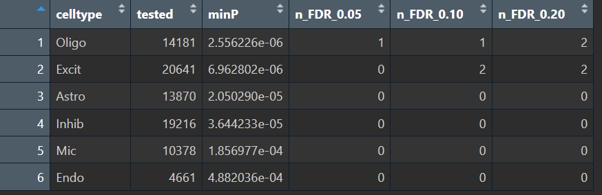
sum_tab <- bind_rows(lapply(cts, \(ct) run_edger_one2(pb_herv_counts, pb_meta, ct))) %>%
arrange(minP)
View(sum_tab)
sum_tab_rna <- bind_rows(lapply(cts, \(ct) run_edger_one2(pb_rna_counts, pb_meta, ct))) %>%
arrange(minP)
View(sum_tab_rna)
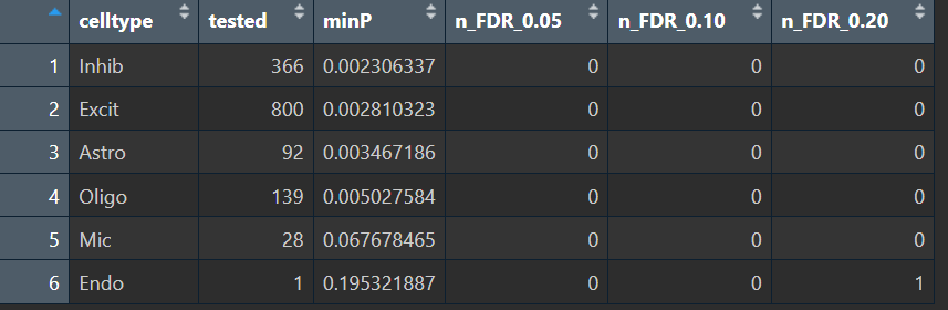
可以看到,我的pseudo-bulk HERV差异结果整体偏弱(在FDR意义下),同时Mic和Endo两类细胞把绝大多数HERV位点都过滤掉了(常见原因:伪bulk库里HERV总计数很低/太稀疏)。说明HERV在这个数据集、这个粒度(6大类)下的稳定差异可能本来就很弱,需要换一种更适合稀疏特征的过滤/检验策略
这说明我们构建pseudo-bulk矩阵+分组+edgeR的流程是没问题的,但RNA在“6大类细胞类型”这个粒度下也整体不显著,说明这个数据在“粗粒度细胞类型+简单group(AD/NC)”下,稳定差异本来就弱,再加上HERV更稀疏,所以更难显著。因此可以先细化差异分析的粒度,比如在某个细胞类型中划分亚群,在亚群中做伪bulk差异
细胞类型亚群level
> table(Idents(scRNA_astro))
  a1   a2   a4  a11   a7   a8  a12   a6  a10   a5   a9   a3
3557 3545 1880  369 1250  940  151 1275  396 1591  469 2683
> table(scRNA_astro$sle_reso, scRNA_astro$group)
        NC   AD
  a1  2011 1546
  a10  367   29
  a11  296   73
  a12   40  111
  a2  1936 1609
  a3   248 2435
  a4  1834   46
  a5    27 1564
  a6   610  665
  a7   631  619
  a8   378  562
  a9    33  436
教程的聚类结果:好像差不太多
  a1   a2   a8   a5   a4   a7   a9   a6   a3
7043 3040  854 1394 1414 1059  550 1321 2445
还是先计算一下富集分数(hERV的差异分析暂时用不到,后面可能用到,这块顺手做一下)
load("C:\\Users\\17185\\Desktop\\hERV_calc\\GSE157827\\my_data\\GSE157827_all_markers_sig.RData")
astro_up <- rownames(subset(all_markers_sig$Astro, avg_log2FC > 0))
astro_down <- rownames(subset(all_markers_sig$Astro, avg_log2FC < 0))
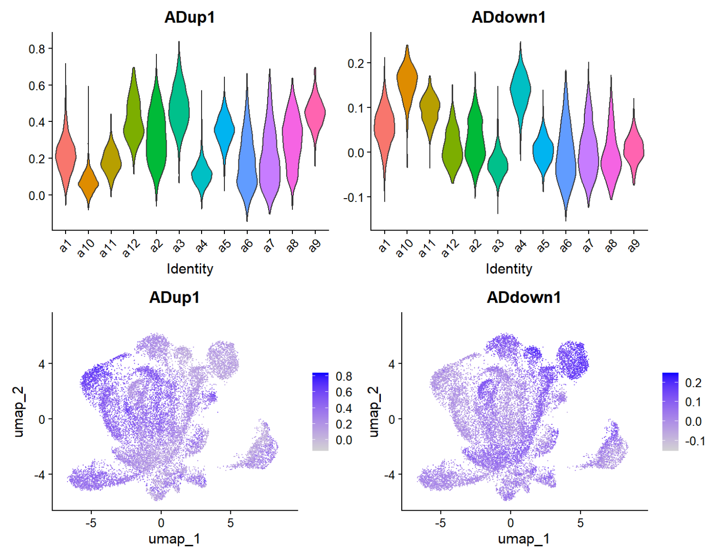
scRNA_astro <- AddModuleScore(scRNA_astro, features = list(astro_up), name = "ADup")
scRNA_astro <- AddModuleScore(scRNA_astro, features = list(astro_down), name = "ADdown")
VlnPlot(scRNA_astro, features = c("ADup1","ADdown1"), group.by = "sle_reso", pt.size = 0) / FeaturePlot(scRNA_astro, features = c("ADup1","ADdown1"))
df <- FetchData(scRNA_astro, vars = c("sle_reso","ADup1","ADdown1","group"))
score_tab <- df %>%
group_by(sle_reso) %>%
summarise(
mean_up = mean(ADup1),
mean_down = mean(ADdown1),
delta = mean_up - mean_down,
n = n()
) %>%
arrange(desc(delta))
View(score_tab)
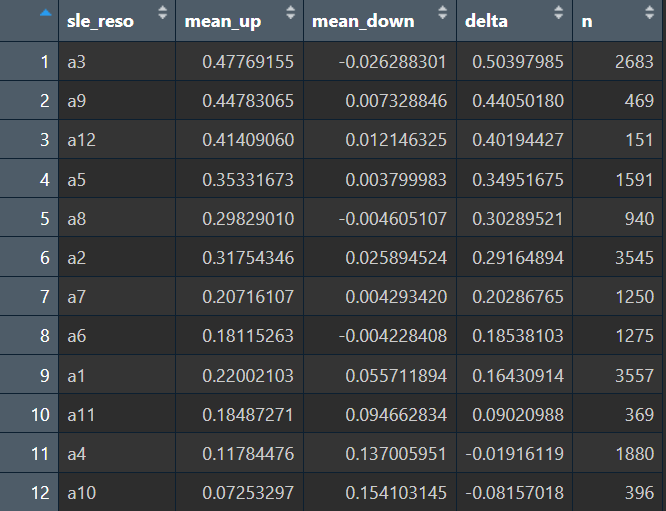
up_core   <- c("a3", "a9", "a12", "a5")
down_core <- c("a4", "a10", "a11")
scRNA_astro$subpop <- "No change"
scRNA_astro$subpop[scRNA_astro$sle_reso %in% up_core]   <- "Up"
scRNA_astro$subpop[scRNA_astro$sle_reso %in% down_core] <- "Down"
scRNA_astro$subpop <- factor(scRNA_astro$subpop, levels=c("Up","Down","No change"))
prop <- prop.table(table(scRNA_astro$sle_reso, scRNA_astro$group), 1)
# 保存数据
saveRDS(
  scRNA_astro,
  file = "C:\\Users\\17185\\Desktop\\hERV_calc\\GSE157827\\my_data\\GSE157827_astro.rds",
  compress = "xz"
)
> table(scRNA_astro$subpop)
       Up      Down No change
     4894      2645     10567
> prop[c(up_core, down_core), ]
              NC         AD
  a3  0.09243384 0.90756616
  a9  0.07036247 0.92963753
  a12 0.26490066 0.73509934
  a5  0.01697046 0.98302954
  a4  0.97553191 0.02446809
  a10 0.92676768 0.07323232
  a11 0.80216802 0.19783198
选出用于hERV差异分析的亚群:
- 如果一个样本在该亚群里≥20细胞,则算做一个有效样本,如果一个亚群的AD/NC有效样本都多于5个,就用这个亚群
- hERV差异分析是否应该在上面得到的差异明显的亚群里做?一个问题是这些亚群往往都只有极少数AD或NC细胞,而pseudo-bulk必须要求样本数够多
- 看来选那些NC-AD数比较均衡的亚群更好?
-
仿照之前教程复现中的做法,根据Up/Down将亚群合并,做Up/Down的hERV差异分析?
然而这种方法也不能回避关键问题:某个样本要么是来自NC,要么是来自AD,而up/down中也是“up的AD多,down的NC多”,导致一个样本无法有足够多的、被划分成up/down的细胞
- 都试一下:
- 路线A:只在“AD/NC两组都有足够样本贡献”的亚群里做表达差异
- 路线B:按Up/Down做“普通单细胞”的HERV差异
先尝试路线A
# 选出适合pseudo-bulk的亚群
min_cells <- 20
min_samples_each_group <- 6
cell_tab <- scRNA_astro@meta.data %>%
  dplyr::transmute(sub = sle_reso, group = group, sample = orig.ident) %>%
  dplyr::count(sub, group, sample, name = "n_cells")
sum_tab <- cell_tab %>%
  dplyr::group_by(sub, group) %>%
  dplyr::summarise(n_samples_ge = sum(n_cells >= min_cells), .groups="drop") %>%
  tidyr::pivot_wider(names_from = group, values_from = n_samples_ge, values_fill = 0) %>%
  dplyr::mutate(keep = (NC >= min_samples_each_group) & (AD >= min_samples_each_group)) %>%
  dplyr::arrange(dplyr::desc(keep), sub)
keep_subs <- sum_tab %>% dplyr::filter(keep) %>% dplyr::pull(sub)
keep_subs  # "a1" "a2" "a6" "a7"
先拿a1做一个小测试
run_pb_herv_one_sub <- function(obj, sub_id, min_cells = 20, min_cpm = 1, min_samp = 3) {
  sub_obj <- subset(obj, subset = sle_reso == sub_id)
  pb_herv <- AggregateExpression(
    sub_obj,
    assays = "HERV",
    slot = "counts",
    group.by = "orig.ident",
    return.seurat = FALSE
  )$HERV
  saminfo <- sub_obj@meta.data %>%
    distinct(orig.ident, group) %>%
    rename(sample = orig.ident) %>%
    filter(sample %in% colnames(pb_herv)) %>%
    arrange(match(sample, colnames(pb_herv)))
  stopifnot(all(saminfo$sample == colnames(pb_herv)))
  saminfo$group <- factor(saminfo$group, levels = c("NC", "AD"))
  print(table(saminfo$group))
  cat("pb_herv dim:", paste(dim(pb_herv), collapse = " x "), "\n")
  y <- DGEList(counts = pb_herv, group = saminfo$group)
  cpm_mat <- cpm(y)
  keep <- (rowSums(cpm_mat[, saminfo$group == "NC", drop=FALSE] > min_cpm) >= min_samp) |
          (rowSums(cpm_mat[, saminfo$group == "AD", drop=FALSE] > min_cpm) >= min_samp)
  y <- y[keep, , keep.lib.sizes = FALSE]
  cat("features kept after CPM filter:", nrow(y), "\n")
  y <- calcNormFactors(y, method = "TMM")
  design <- model.matrix(~ group, data = saminfo)
  y <- estimateDisp(y, design, robust = TRUE)
  fit <- glmQLFit(y, design, robust = TRUE)
  qlf <- glmQLFTest(fit, coef = "groupAD")
  res <- topTags(qlf, n = Inf)$table %>%
    tibble::rownames_to_column("feature")
  cat("min PValue:", min(res$PValue), "\n")
  cat("min FDR  :", min(res$FDR), "\n")
  cat("FDR<0.05:", sum(res$FDR < 0.05), "\n")
  cat("FDR<0.10:", sum(res$FDR < 0.10), "\n")
  cat("FDR<0.20:", sum(res$FDR < 0.20), "\n")
  list(res = res, pb = pb_herv, saminfo = saminfo)
}
out_a1 <- run_pb_herv_one_sub(scRNA_astro, sub_id = "a1")
View(out_a1$res)
NC AD
 9 11
pb_herv dim: 4326 x 20
features kept after CPM filter: 405
min PValue: 0.0004331899
min FDR  : 0.122591
FDR<0.05: 0
FDR<0.10: 0
FDR<0.20: 4
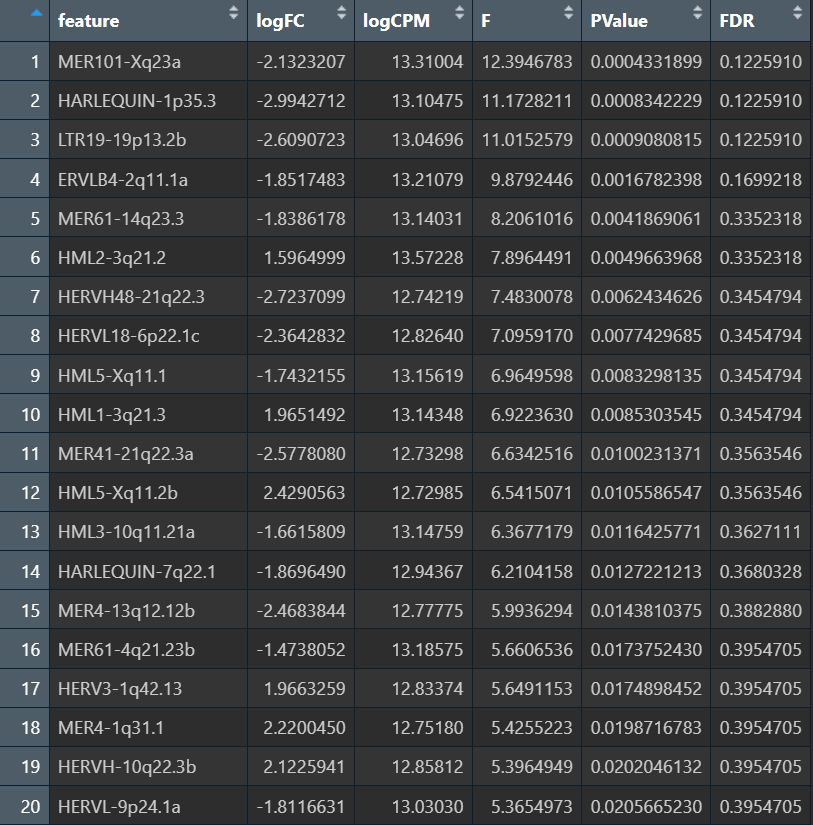
因为调整了feature的过滤方法,所以filterByExpr后剩下405个,比较正常。FDR最小为0.1226,在“稀疏+多重检验+效应可能不大”的场景下还算合理(HERV在样本间离散度大、且很多feature在一部分样本几乎0),因此现在能看到一些候选,但还不足以说强显著
因为hERV太稀疏,所以还要看是不是少数样本/outlier值影响了结果
最后确实得到的结果FDR都有些太大了,虽然经过检验(画小提琴图展示样本计数分布、leave-one-out重新计算)很多信号不是被某一个样本单点“拽出来”的那种极端情况,但不同样本对显著性会有影响
尝试路线B
在之前的教程中,我们在“找Up-Down的差异基因并GO富集”的步骤中:
marker_Astro <- FindMarkers(
  scRNA_astro_sub,
  group.by = "subpop",
  ident.1 = "Down",
  ident.2 = "Up"
)
marker_Astro <- marker_Astro[order(marker_Astro$p_val_adj, decreasing = F), ]
marker_Astro_sig <-  marker_Astro %>%
  rownames_to_column("gene") %>%
  filter(p_val_adj < 0.05, abs(avg_log2FC) >= 0.25) %>%
  filter(pct.1 >= 0.1 | pct.2 >= 0.1) %>%
  filter(!grepl("^(ENSG|MT-|LINC)|^(AC|AL)[0-9]", gene))
这里先简单参照一下
scUD <- readRDS("C:\\Users\\17185\\Desktop\\hERV_calc\\GSE157827\\my_data\\GSE157827_astro_sub.rds")
DefaultAssay(scUD) <- "HERV"
Idents(scUD) <- "subpop"
# Wilcoxon:不校正协变量
mk_wilcox <- FindMarkers(
  scUD,
  ident.1 = "Up", ident.2 = "Down",
  test.use = "wilcox",
  logfc.threshold = 0.5,
  min.pct = 0.01
)
View(mk_wilcox %>% arrange(p_val_adj))
# MAST:把“样本/库深度/线粒体”等作为协变量
mk_mast <- FindMarkers(
  scUD,
  ident.1 = "Up", ident.2 = "Down",
  test.use = "MAST",
  latent.vars = c("orig.ident", "nCount_RNA", "percent_mito"),
  logfc.threshold = 0.5,
  min.pct = 0.01
)
View(mk_mast %>% arrange(p_val_adj))
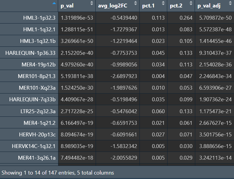
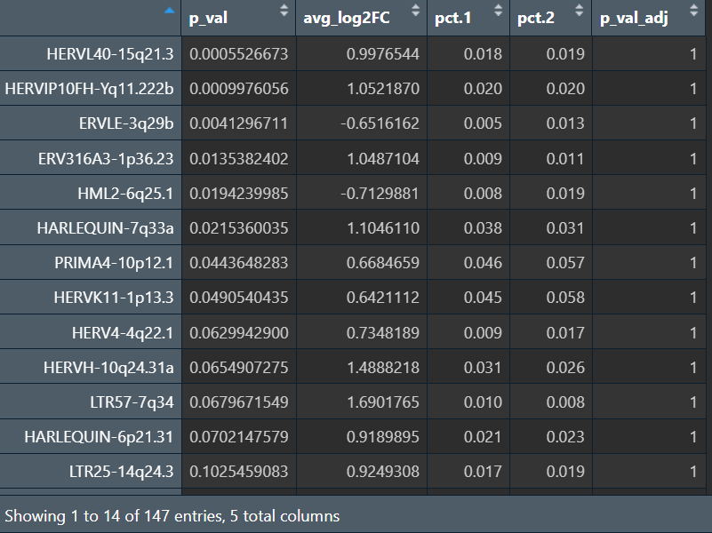
因为如果把样本作为协变量,由于每个样本内不可能同时有大量的AD和NC细胞,所以p_adj就变成了1
虽然教程里是这么做的,但GPT提出了一个问题:up-down的状态差异是否等于AD-NC的疾病差异,是否应该“在同一亚群/同一状态内比较(比如路线A)”,或者只在AD/NC内比较Up-Down,如果某些hERV确实是疾病差异,应该在多个亚群内都能看到一致方向的AD-NC差异
细胞轨迹test
简介
以“Monocle3/Slingshot/tradeSeq”这三种工具为例
简单来说:
- Monocle3:想把细胞排序(例如构建pseudotime),并得到分支/主干结构。适合发育/分化、免疫激活连续谱、应激/反应性渐变等情况
- Slingshot:已经有Seurat聚类(UMAP/PCA),只想在这个结构上找主线/分支。适合亚群内连续谱(而不是“从零建图”)
-
tradeSeq:给定pseudotime(来自Monocle/Slingshot等),对每个基因拟合GAM平滑曲线,然后做统计检验,回答“表达随状态轴如何变化、组间曲线是否不同”的问题,即“把轨迹变成可检验的差异结论”
所以,Monocle3和Slingshot是上游分析,tradeSeq是下游分析
Monocle3:降维 → learn_graph → order_cells → pseudotime
- 轨迹骨架(principal graph):不是简单连cluster,而是试图在低维空间里学出一条“主干+分支”的结构
- pseudotime:每个细胞在骨架上的位置,只代表“顺序/相对位置”,不等价真实时间,需要root(起点)
- 分支/分区(partition/branch):把结构分成若干区域,分支点附近常有“状态转换”意义,每个分支不一定是“真实生物学分化”,有时是UMAP/图学习导致的结构
- 相比Slingshot,如果想要得到骨架图(像发育谱系那样),或者认为之前得到的聚类不完全准确、不想完全依赖聚类拓扑,就使用Monocle3
Slingshot:低维坐标(PCA/UMAP)+ cluster标签 → 在聚类间构建连接结构 → 在细胞层面拟合principal curves得到轨迹
- 路径(Lineage):在“从起点cluster出发”的拓扑下,存在多个可能终点/分支路径
-
pseudotime矩阵(pt_mat):cells × lineages,每个细胞在每条lineage上都有一个pseudotime,如果不属于该路径就是NA
一个细胞可能只属于某一条路径,也可能在分支附近对多条路径都有一定归属
- cellWeights矩阵(cw_mat):cells × lineages,这个细胞对某条lineage的归属程度/权重,分支点附近的细胞可能对两条lineage都有权重
- 相比Monocle3,如果已经有准确聚类,且“状态谱”更多是聚类的连续过渡,希望轨迹推断对聚类结构更稳健,就使用Slingshot
tradeSeq:
- 输入:
- 原始计数矩阵
- pseudotime:来自Monocle/Slingshot等
- cellWeights:存在分支、有多条路径时很重要
- conditions:如AD/NC,用来比较曲线
- 输出:拟合模型对象gam——每个基因都有一条(或多条lineage × condition的)平滑表达曲线模型
- 常用检验:
-
associationTest(gam):这个基因是否随pseudotime变化,适合找“状态轴上的标志基因/动态基因” -
conditionTest(gam):AD-NC的曲线形状/水平是否不同,组间在轨迹上是否不同步/不同形态 -
startVsEndTest(gam):起点与终点是否显著不同,体现稳态与反应态的差异 -
earlyDETest(gam):两组在轨迹早期就分开了吗(“早期偏移”) -
diffEndTest(gam):不同分支终点的表达是否不同(分支终末态比较)
-
总结:
- Monocle3:在该细胞类型内部学习到一条(或多条分支的)连续状态轨迹;伪时间刻画了从稳态向反应/应激态的连续过渡
- Slingshot:基于聚类拓扑与低维嵌入,拟合得到若干条潜在状态路径;细胞在主路径上的伪时间可用于描述状态推进,并用于下游动态分析
- tradeSeq:沿伪时间拟合表达平滑曲线,识别出显著随轨迹变化的基因,以及在AD与NC间轨迹动态显著不同的基因/模块,提示疾病改变了同一状态轴上的转变过程
以astro细胞为例,直接使用之前已完成预处理的Seurat对象
Monocle3的pseudotime
数据准备
library(Seurat)
library(tidyverse)
library(patchwork)
scRNA <- readRDS("C:\\Users\\17185\\Desktop\\hERV_calc\\GSE157827\\data\\GSE157827_astro.rds")
res_dir <- "C:\\Users\\17185\\Desktop\\hERV_calc\\GSE157827\\res"
pseudotime分析
library(monocle3)
expr <- GetAssayData(scRNA, slot = "counts")
cell_meta <- scRNA@meta.data
gene_meta <- data.frame(
  gene_short_name = rownames(expr),
  row.names = rownames(expr)
)
cds <- new_cell_data_set(
  expr,
  cell_metadata = cell_meta,
  gene_metadata = gene_meta
)
# 直接使用Seurat的UMAP结果
reducedDims(cds)$UMAP <- Embeddings(scRNA, "umap")
cds <- cluster_cells(cds, reduction_method = "UMAP")
# 学习轨迹图
cds <- learn_graph(cds, use_partition = TRUE)
# try1:用braak.tangle.stage最小的细胞当root
earliest <- min(scRNA$braak.tangle.stage, na.rm = TRUE)
root_cells <- colnames(scRNA)[which(scRNA$braak.tangle.stage == earliest)]
# 排序
cds <- order_cells(cds, root_cells = root_cells)
pt <- monocle3::pseudotime(cds)
# 写回Seurat
scRNA$pseudotime <- pt[colnames(scRNA)]
# 轨迹与分组分布
FeaturePlot(scRNA, features = "pseudotime")  # 看轨迹轴在UMAP上的走向
VlnPlot(scRNA, features = "pseudotime", group.by = "group", pt.size = 0)
VlnPlot(scRNA, features = "pseudotime", group.by = "braak.tangle.stage", pt.size = 0)
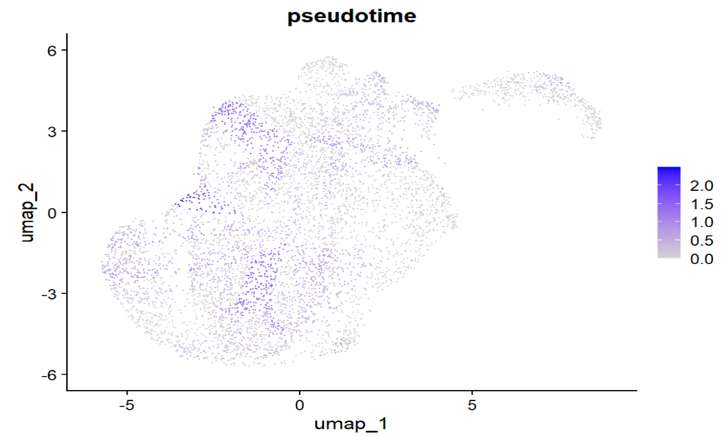
似乎不是“整张UMAP从一端平滑过渡到另一端”的那种形态,大部分都接近0,只有小部分有颜色
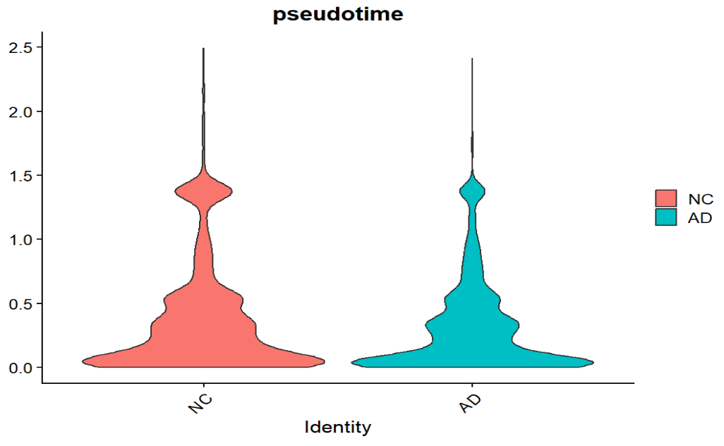
与上张图分布相似,两组都大量堆在接近0的位置,只有少量细胞在1–2.5的尾部,说明pseudotime的“有效动态范围”只覆盖了一小部分细胞,所以组间整体差异不容易被拉开
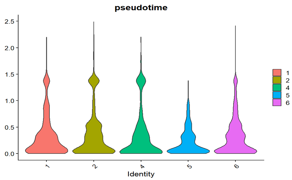
stage也都是大量细胞集中在低pseudotime,且stage之间没有非常清晰的“随分期单调递增”的趋势,说明当前这条pseudotime轴与Braak分期的对齐程度不强,不能得出“AD一定更反应/更晚期”的结论
- 提示root可能选的过宽(我在6000细胞中选择600个分期最早的作为root),导致pseudotime本身就不太像“单一方向的进程”
- Braak是样本级标签+分期不一定覆盖连续状态+样本间异质性大,导致不构成稳定梯度
# 单基因平滑曲线
genes <- c("SLC1A2","ALDH1L1","GFAP")
df <- FetchData(scRNA, vars = c("pseudotime","group", genes))
df_long <- pivot_longer(df, cols = all_of(genes), names_to = "gene", values_to = "expr")
ggplot(df_long, aes(x = pseudotime, y = expr, color = group)) +
  geom_point(size = 0.2, alpha = 0.2) +
  geom_smooth(se = FALSE, method = "loess", span = 0.3) +
  facet_wrap(~gene, scales = "free_y") +
  theme_classic()
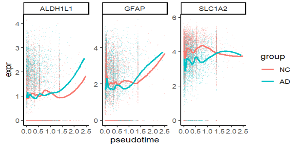
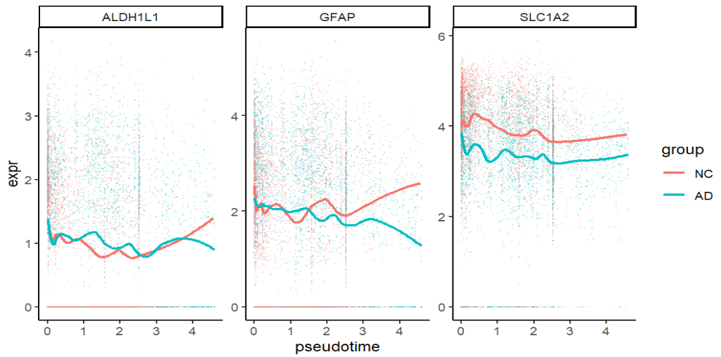
GFAP逐渐上升、SLC1A2较平(理论上应该下降)、ALDH1L1逐渐上升(确实是表达增强,但可能受技术因素影响),说明pseudotime与astro某些状态变化有关
可能的原因:用earliest分期的大量细胞当root,导致root覆盖太广,所以绝大多数细胞的pseudotime接近0,只有离这些root都远的一部分区域出现高pseudotime
考虑到之前的分析中,我们在差异基因中选了最top的一些计算了模块分数,能不能用这个模块分数来辅助选root
# 用之前得到的划分好up/down的astro
scRNA_astro_sub <- readRDS("C:\\Users\\17185\\Desktop\\hERV_calc\\GSE157827\\data\\GSE157827_astro_sub.rds")
scRNA_astro_sub$subpop <- factor(scRNA_astro_sub$subpop, levels = c("Down","Up"))
marker_Astro <- FindMarkers(
  scRNA_astro_sub,
  group.by = "subpop",
  ident.1 = "Down",
  ident.2 = "Up"
)
marker_Astro <- marker_Astro[order(marker_Astro$p_val_adj, decreasing = F), ]
marker_Astro_sig <- marker_Astro %>%
  rownames_to_column("gene") %>%
  filter(p_val_adj < 0.05, abs(avg_log2FC) >= 0.25) %>%
  filter(pct.1 >= 0.1 | pct.2 >= 0.1) %>%
  filter(!grepl("^(ENSG|MT-|LINC)|^(AC|AL)[0-9]", gene))
# Down子群体更高表达的基因
astro_down <- marker_Astro_sig %>%
  filter(avg_log2FC > 0) %>%
  arrange(p_val_adj, desc(abs(avg_log2FC))) %>%
  slice_head(n = 20) %>%
  pull(gene)
# Up子群体更高表达的基因
astro_up <- marker_Astro_sig %>%
  filter(avg_log2FC < 0) %>%
  arrange(p_val_adj, desc(abs(avg_log2FC))) %>%
  slice_head(n = 20) %>%
  pull(gene)
scRNA <- AddModuleScore(scRNA, features = list(astro_up), name = "ADup")
scRNA <- AddModuleScore(scRNA, features = list(astro_down), name = "ADdown")
FeaturePlot(scRNA, features = c("ADup1","ADdown1"))
VlnPlot(scRNA, features = c("ADup1","ADdown1"), group.by="group", pt.size=0)
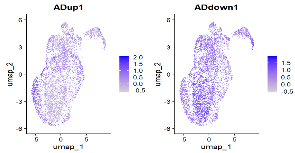
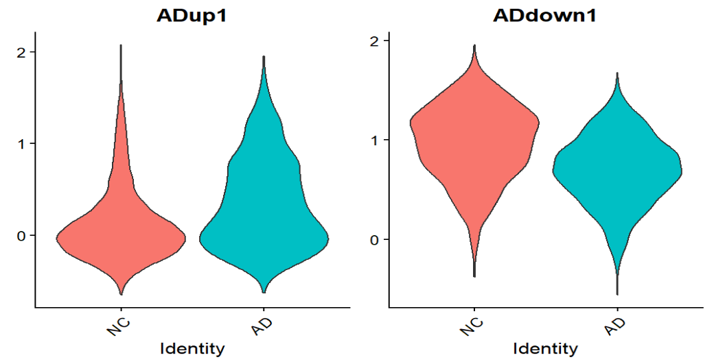
在ADup和ADdown的层面,确实是形成了“状态区域”,也证明astro里确实存在“疾病相关表达程序”的整体偏移,提示可以使用up/down的模块分数来选root
try2:使用模块分数选出稳态端当root
- 稳态端:ADup1低+ADdown1高
- 反应端:ADup1高+ADdown1低
root_score <- scale(scRNA$ADdown1) - scale(scRNA$ADup1)
names(root_score) <- colnames(scRNA)
# 在earliest分期中
scRNA$braak_num <- suppressWarnings(as.numeric(as.character(scRNA$braak.tangle.stage)))
earliest <- min(scRNA$braak_num, na.rm = TRUE)
cand <- colnames(scRNA)[scRNA$braak_num == earliest]
# 取最稳态的前200个
cand <- cand[order(root_score[cand], decreasing = TRUE)]
root_cells <- head(cand, 200)
# 只要一条主轴
cds <- learn_graph(cds, use_partition = FALSE)
cds <- order_cells(cds, root_cells = root_cells)
scRNA$pseudotime <- monocle3::pseudotime(cds)[colnames(scRNA)]
# 画图代码同上
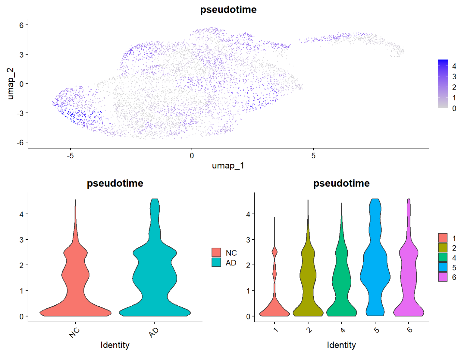
- 可以看到,umap图上变蓝的部分更多,AD-NC的pseudotime差异也更明显(AD更富集在“后段状态”),同时braak分期更晚的pseudotime更高(说明这条轴与braak有一定相关性)
- SLC1A2随pseudotime变化不明显,GFAP后端状态与预期不符,可能是pseudotime高的细胞数在AD/NC不均衡,导致曲线在尾部容易被少量点带偏
想看一下“模块分数随pseudotime的趋势”
df <- FetchData(obj, vars = c("pseudotime", "group", "ADup1", "ADdown1")) %>%
  filter(!is.na(pseudotime))
df_long <- df %>%
  pivot_longer(cols = c("ADup1", "ADdown1"), names_to = "module", values_to = "score")
# 相关系数
cor.test(df$pseudotime, df$ADup1, method = "spearman")  # 总体相关
cor.test(df$pseudotime, df$ADdown1, method = "spearman")
df %>% group_by(group) %>%  # 分组相关
  summarise(
    rho_ADup   = cor(pseudotime, ADup1, method = "spearman"),
    rho_ADdown = cor(pseudotime, ADdown1, method = "spearman"),
    .groups = "drop"
  )
# LOESS平滑曲线
ggplot(df_long, aes(x = pseudotime, y = score, color = group)) +
  geom_point(size = 0.2, alpha = 0.12) +
  geom_smooth(se = FALSE, method = "loess", span = 0.35) +
  facet_wrap(~module, scales = "free_y") +
  theme_classic()
# 分箱均值曲线(避免尾部LOESS被少量点带偏)
df_long <- df_long %>%
  mutate(pt_bin = ggplot2::cut_number(pseudotime, n = 30))
sum_tab <- df_long %>%
  group_by(group, module, pt_bin) %>%
  summarise(
    pt_mid = mean(pseudotime),
    score_mean = mean(score),
    n = dplyr::n(),
    .groups = "drop"
  )
ggplot(sum_tab, aes(x = pt_mid, y = score_mean, color = group)) +
  geom_line() +
  geom_point(aes(size = n), alpha = 0.8) +
  facet_wrap(~module, scales = "free_y") +
  theme_classic() +
  guides(size = "none")
data:  df$pseudotime and df$ADup1
S = 3.3663e+10, p-value < 2.2e-16
alternative hypothesis: true rho is not equal to 0
sample estimates:
      rho
0.2405992

data:  df$pseudotime and df$ADdown1
S = 5.5218e+10, p-value < 2.2e-16
alternative hypothesis: true rho is not equal to 0
sample estimates:
       rho
-0.2456553

group  rho_ADup  rho_ADdown
NC	0.07784422	-0.2370371
AD	0.33427566	-0.1747888
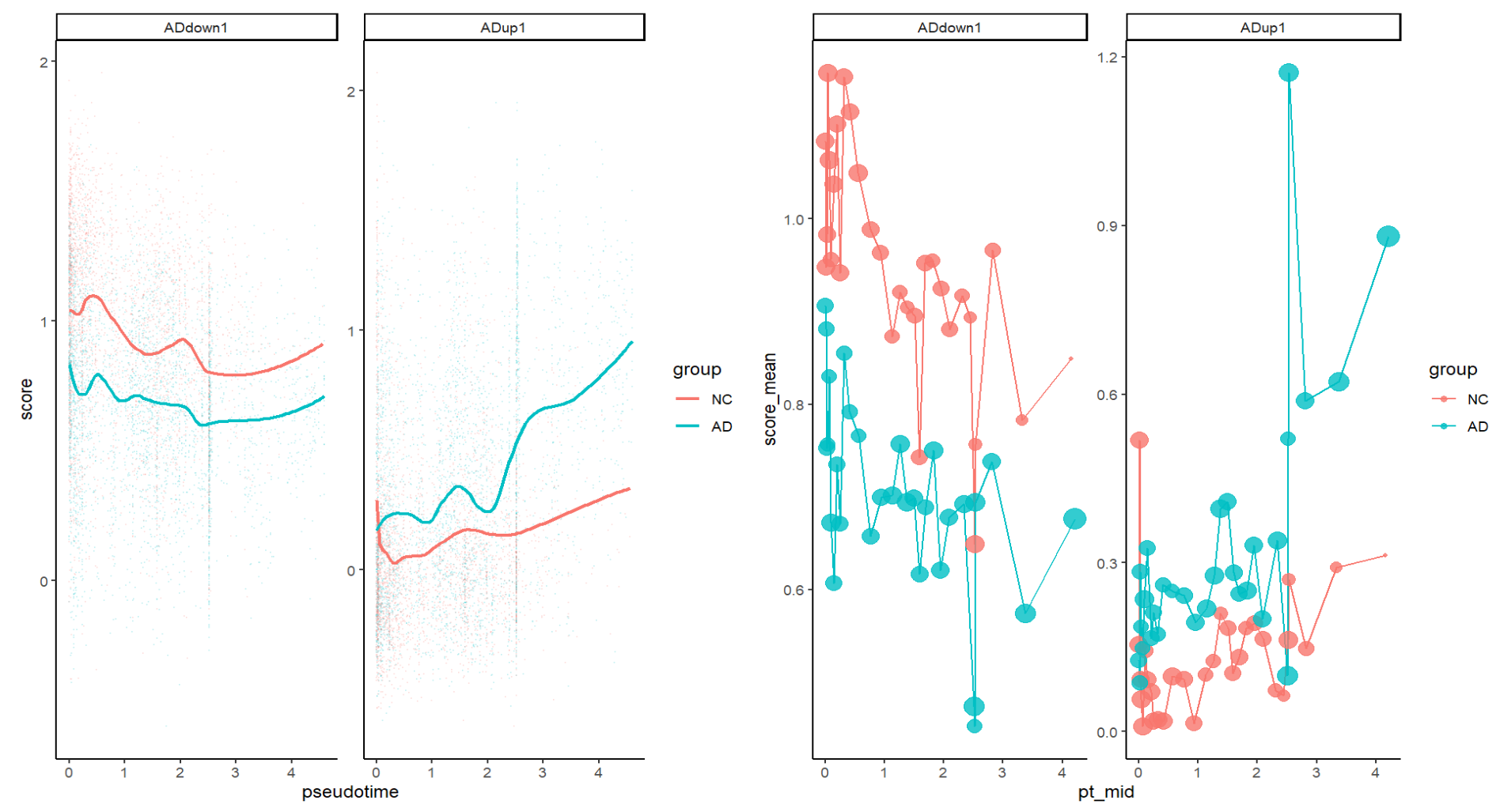
- ADdown1:NC全程都高于AD,并随pseudotime整体缓慢下降(ADdown基因集作为稳态/保护/对照端程序,在“后段状态”逐渐变弱
- ADup1:AD在pseudotime后段明显上升,且上升幅度较NC更大(ADup基因集在“后段状态”增强,而且主要发生在AD细胞里)
- 相关系数的方向符合预期,rho值小说明“有信号但不是一条单因素决定的轴”(在AD这种复杂疾病状态谱里很正常)
- 分组相关系数说明这条pseudotime轴更能捕捉“AD中出现的反应/疾病相关程序的进行”
Slingshot+tradeSeq
数据准备:读取之前的Seurat对象并添加ADup和ADdown分数
library(Seurat)
library(tidyverse)
library(patchwork)
library(SingleCellExperiment)
library(slingshot)
library(tradeSeq)
library(scater)
res_dir <- "C:\\Users\\17185\\Desktop\\hERV_calc\\GSE157827\\res"
sceu <- readRDS("C:\\Users\\17185\\Desktop\\hERV_calc\\GSE157827\\data\\GSE157827_astro.rds")
sceu_astro_sub <- readRDS("C:\\Users\\17185\\Desktop\\hERV_calc\\GSE157827\\data\\GSE157827_astro_sub.rds")
sceu_astro_sub$subpop <- factor(sceu_astro_sub$subpop, levels = c("Down","Up"))
marker_Astro <- FindMarkers(
  sceu_astro_sub,
  group.by = "subpop",
  ident.1 = "Down",
  ident.2 = "Up"
)
marker_Astro <- marker_Astro[order(marker_Astro$p_val_adj, decreasing = F), ]
marker_Astro_sig <- marker_Astro %>%
  rownames_to_column("gene") %>%
  filter(p_val_adj < 0.05, abs(avg_log2FC) >= 0.25) %>%
  filter(pct.1 >= 0.1 | pct.2 >= 0.1) %>%
  filter(!grepl("^(ENSG|MT-|LINC)|^(AC|AL)[0-9]", gene))
astro_down <- marker_Astro_sig %>%
  filter(avg_log2FC > 0) %>%
  arrange(p_val_adj, desc(abs(avg_log2FC))) %>%
  slice_head(n = 20) %>%
  pull(gene)
astro_up <- marker_Astro_sig %>%
  filter(avg_log2FC < 0) %>%
  arrange(p_val_adj, desc(abs(avg_log2FC))) %>%
  slice_head(n = 20) %>%
  pull(gene)
sceu <- AddModuleScore(sceu, features = list(astro_up), name = "ADup")
sceu <- AddModuleScore(sceu, features = list(astro_down), name = "ADdown")
Seurat对象 → SingleCellExperiment对象 → 使用Slingshot建轨迹+pseudotime
sce <- as.SingleCellExperiment(sceu)
reducedDim(sce, "UMAP") <- Embeddings(sceu, "umap")
clus <- sceu$seurat_clusters
# 根据上回的经验,直接用更ADdown的细胞做起始cluster
score <- sceu$ADdown1 - sceu$ADup1
tab0 <- data.frame(cl = clus, score = score, group = sceu$group) %>%
group_by(cl) %>%
summarise(score_med = median(score, na.rm = TRUE),
nc_prop = mean(group == "NC", na.rm = TRUE),
n = n(), .groups="drop") %>%
arrange(desc(score_med), desc(nc_prop))
start_clus <- as.character(tab0$cl[1])
# slingshot
sce <- slingshot(
sce,
clusterLabels = "seurat_clusters",
reducedDim = "UMAP",
start.clus = start_clus
)
# UMAP + 轨迹曲线
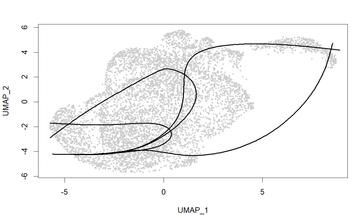
plot(reducedDim(sce, "UMAP"), col = "grey80", pch = 16, cex = 0.4,
xlab = "UMAP_1", ylab = "UMAP_2")
lines(SlingshotDataSet(sce), lwd = 2, col = "black")
# pseudotime(如果多条轴,先用第一条/主线)
pt_mat <- slingPseudotime(sce)
cw_mat <- slingCurveWeights(sce)
sceu$pseudotime_sling <- pt_mat[, 1]
> ncol(slingPseudotime(sce))
[1] 4
> table(sceu$seurat_clusters)
   0    1    2    3    4    5    6    7    8
1799 1457  805  621  545  476  427  184  117
这说明有4条可行的主路径(分支或不同终点),同时UMAP图中的曲线有交叉和回环,可能是因为UMAP的几何会扭曲全局结构(因此也有一种做法是在PCA空间中进行Slingshot),同时cluster分的较细且彼此连接关系复杂,导致Slingshot会给出多条可能路径,这里通常就需要选一条“最像反应性/激活轴”的主线来解释,这里为了简单测试就直接取了第一条,如果想认真选的话,可以用cellWeights统计每条lineage覆盖的细胞数,选覆盖最多的一条当主线,并只用这一条做后面的tradeSeq
# pseudotime是否与ADup/ADdown对齐
FeaturePlot(sceu, "pseudotime_sling") | VlnPlot(sceu, "pseudotime_sling", group.by = "group", pt.size = 0)
# 模块分数随pseudotime的趋势(辅助解释轨迹方向)
df <- FetchData(sceu, vars = c("pseudotime_sling","group","ADup1","ADdown1")) %>%
  filter(!is.na(pseudotime_sling))
df_long <- df %>%
  pivot_longer(cols = c("ADup1","ADdown1"), names_to = "module", values_to = "score") %>%
  mutate(pt_bin = ggplot2::cut_number(pseudotime_sling, n = 30))
sum_tab <- df_long %>%
  group_by(group, module, pt_bin) %>%
  summarise(
    pt_mid = mean(pseudotime_sling),
    score_mean = mean(score),
    n = n(),
    .groups = "drop"
  ) %>%
  filter(n >= 50)  # 可改 30/50/100
p1 <- ggplot(sum_tab, aes(x = pt_mid, y = score_mean, color = group)) +
  geom_line() +
  geom_point(aes(size = n), alpha = 0.8) +
  facet_wrap(~module, scales = "free_y") +
  theme_classic() +
  guides(size = "none")
# 样本级分析
meta <- FetchData(sceu, vars = c("pseudotime_sling","group","orig.ident")) %>%
  filter(!is.na(pseudotime_sling))
sample_tab <- meta %>%
  group_by(orig.ident, group) %>%
  summarise(pt_median = median(pseudotime_sling),
            pt_mean = mean(pseudotime_sling),
            .groups="drop")
wilcox.test(pt_median ~ group, data = sample_tab)
p2 <- ggplot(sample_tab, aes(x = group, y = pt_median)) +
  geom_boxplot(outlier.shape = NA) +
  geom_jitter(width = 0.15, height = 0) +
  theme_classic()
p1 | p2
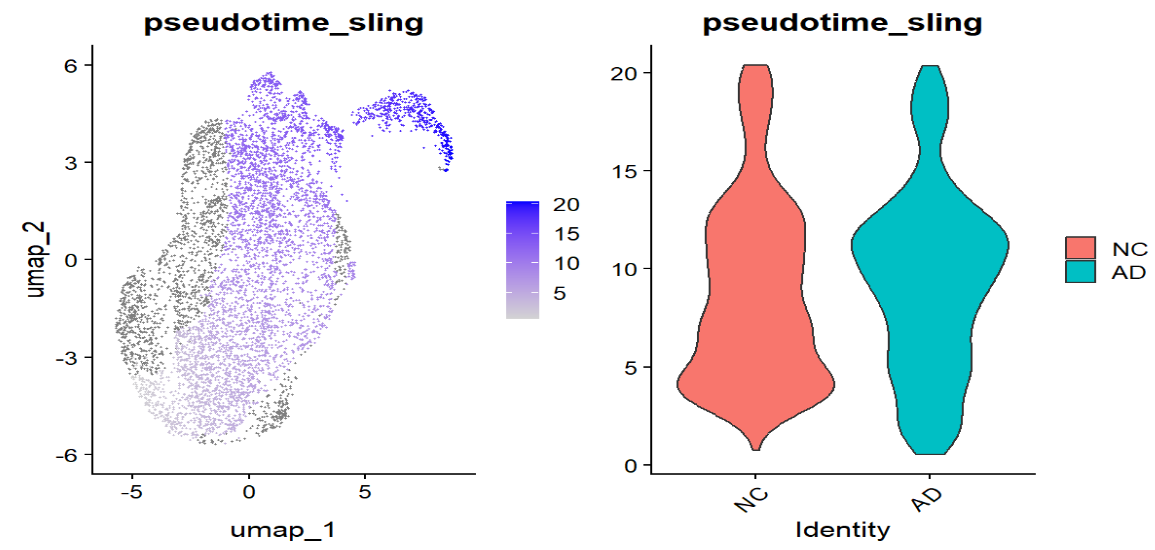
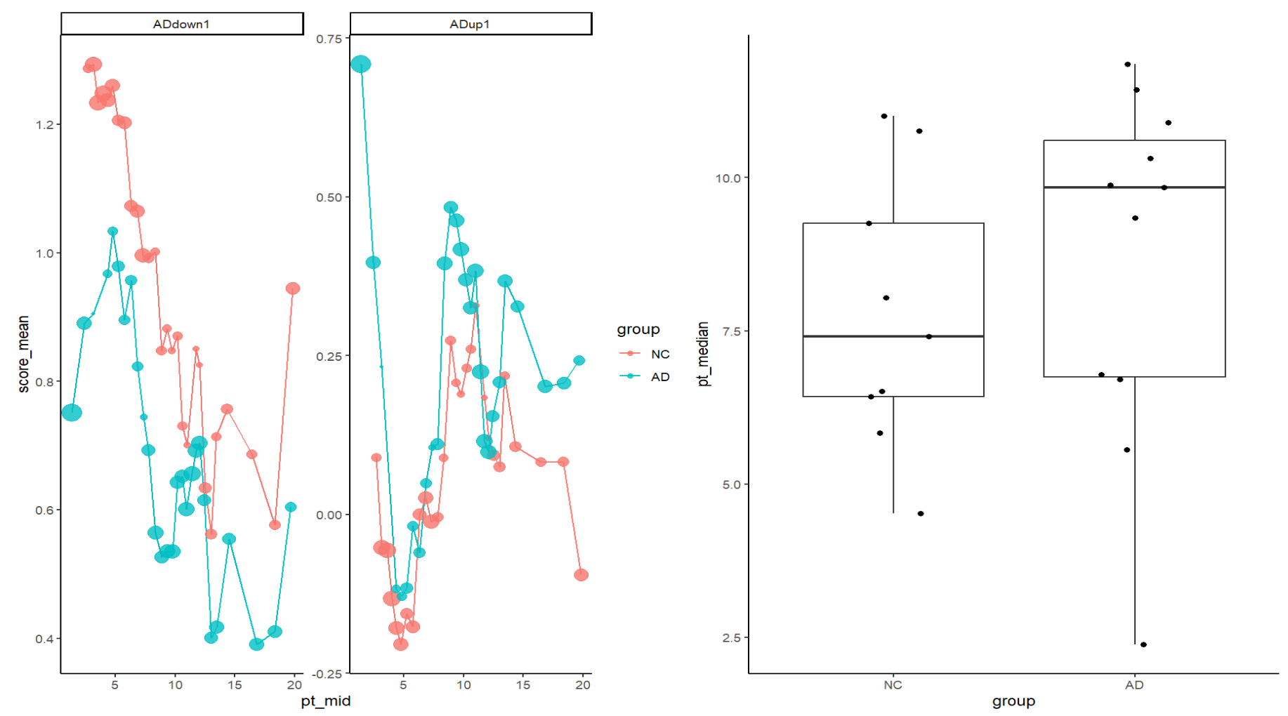
这里的结果和上面monocle3的类似(AD与NC的细胞分布存在偏移,并且与ADup/ADdown模块分数呈一致的趋势变化),说明选的这条线路很可能是在刻画“稳态 → 反应/应激”的连续变化
tradeSeq:轨迹上“变化基因”与“AD/NC 曲线不同”的基因
# 准备counts+选择基因集合(这里作为测试只使用HVG)
use_genes <- VariableFeatures(sceu)
counts <- GetAssayData(sceu, slot = "counts")[use_genes, ]
# 过滤NA
pt1 <- pt_mat[, 1, drop = FALSE]
cw1 <- cw_mat[, 1, drop = FALSE]
keep <- !is.na(pt1[,1]) & (cw1[,1] > 0)
counts2 <- counts[, keep]
pt1_2   <- pt1[keep, , drop = FALSE]
cw1_2   <- cw1[keep, , drop = FALSE]
cond2   <- factor(sceu$group[keep])
# 拟合GAM
cond <- sceu$group
set.seed(1)
gam <- fitGAM(
  counts = counts2,
  pseudotime = pt1_2,
  cellWeights = cw1_2,
  conditions = cond2,
  nknots = 6,
  verbose = TRUE
)
# 哪些基因沿轨迹变化(不分组)
asso <- associationTest(gam)
asso <- asso[order(asso$pvalue), ]
# 哪些基因在轨迹上AD/NC曲线不同
ct <- conditionTest(gam)
ct <- ct[order(ct$pvalue), ]
-
associationTest:找沿轨迹变化的基因(基础轨迹信号) -
conditionTest:找“同一轨迹位置上,AD-NC表达曲线不同”的基因(疾病差异)
> head(asso, 10)
            waldStat df pvalue meanLogFC
KCNIP4     2119.4446 11      0 1.1746620
CSMD1      1911.0154 11      0 1.1147822
SYT1       1920.7033 11      0 1.3592505
AC109466.1  266.5855 11      0 1.2754283
ATRNL1     1310.6656 11      0 1.8489925
SNTG1      1336.8417 11      0 1.1888490
HS6ST3      996.8393 11      0 2.2509793
NRXN3      2272.4418 11      0 1.8331828
RIMS2      1343.5195 11      0 1.5773849
NEGR1       839.9709 11      0 0.7599727
> head(ct, 10)
         waldStat df pvalue
KCND2    90.97927  6      0
CADPS   117.12250  6      0
DPP10   170.40654  6      0
AGBL4   150.26273  6      0
MT-CO3   89.87541  6      0
MT-ATP6 208.06991  6      0
MT-CO2  148.37502  6      0
PHACTR1  99.24620  6      0
MT-ND3  196.30111  6      0
MT-ND4  118.87843  6      0
# top基因在轨迹上的平滑曲线
top_asso <- rownames(asso)[1:6]
top_ct   <- rownames(ct)[1:6]
association_top_genes <- plotSmoothers(gam, counts, gene = top_asso, alpha = 1)
conditionTest_top_genes <- plotSmoothers(gam, counts, gene = top_ct, alpha = 1)
association_top_genes | conditionTest_top_genes
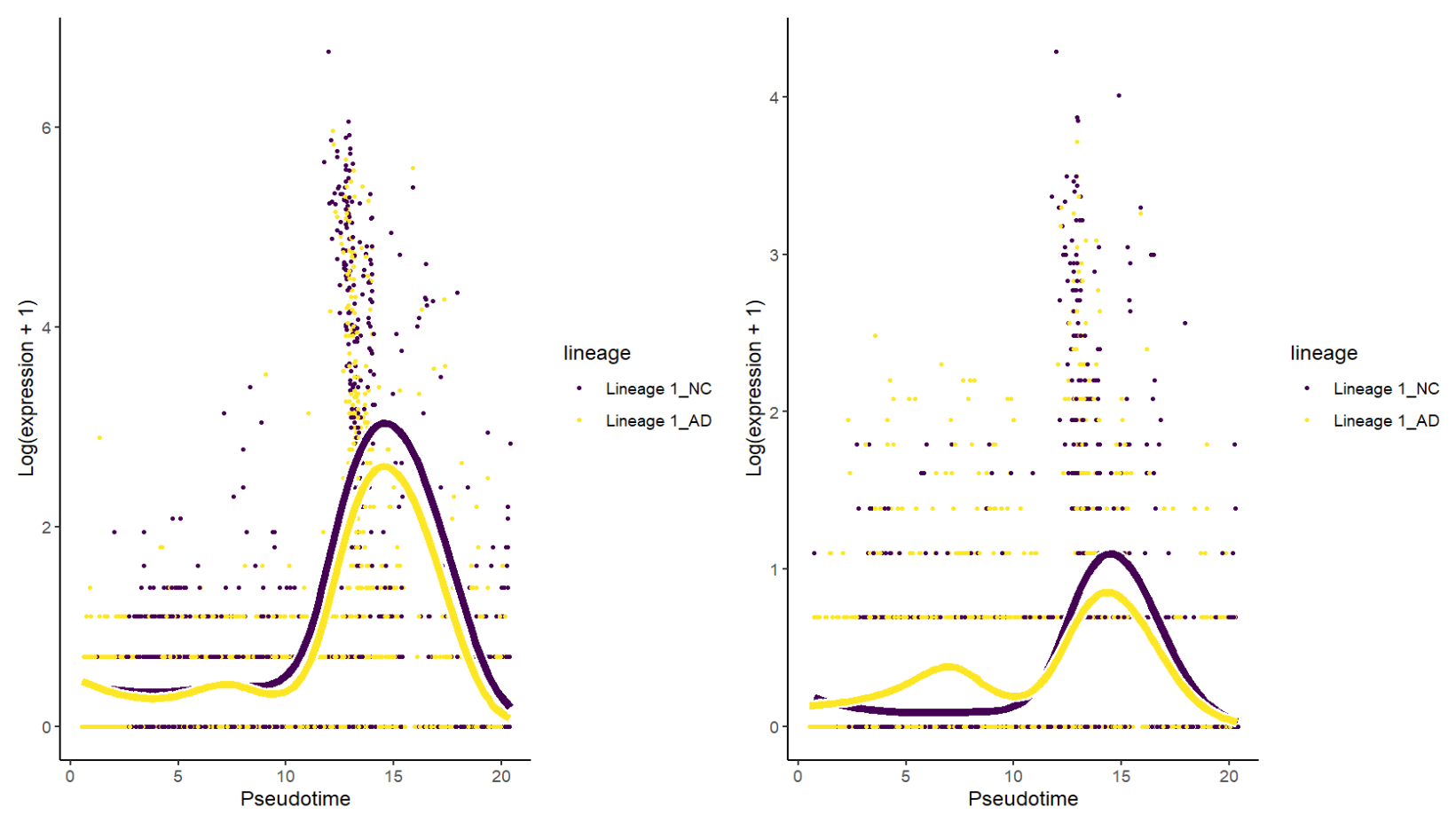
这里得到的top基因很多都是神经元/突触相关基因,可能是因为细胞集内混入了神经元/双细胞/环境RNA,或者技术差异(比如线粒体基因含量)的影响。如果后续要进行分析,可能要剔除掉有“污染/双细胞”的cluster