使用我的GSE157827数据进行初步分析-2
other-other2026.1.15-2026.1.28研究进展
计算family-level计数矩阵
library(Seurat)
library(tidyverse)
library(ggpubr)
library(ggrepel)
library(patchwork)
library(Matrix)
library(edgeR)
library(clusterProfiler)
library(org.Hs.eg.db)
library(MAST)
library(SingleCellExperiment)
res_dir <- "C:\\Users\\17185\\Desktop\\hERV_calc\\GSE157827\\my_res"
seu <- readRDS("C:\\Users\\17185\\Desktop\\hERV_calc\\GSE157827\\my_data\\GSE157827_celltype.rds")
# seu <- readRDS("C:\\Users\\17185\\Desktop\\hERV_calc\\GSE157827\\my_data\\GSE157827_astro.rds")
# seu <- readRDS("C:\\Users\\17185\\Desktop\\hERV_calc\\GSE157827\\my_data\\GSE157827_astro_sub.rds")
herv_loc <- GetAssayData(seu, assay = "HERV", layer = "counts")
feat <- rownames(herv_loc)
if(feat[1] == "--no-feature"){
  feat[1] <- "noFeature"
}
fam <- ifelse(grepl("-", feat), sub("-.*$", "", feat), feat)
fam <- factor(fam)
G <- Matrix::sparse.model.matrix(~ 0 + fam)
colnames(G) <- levels(fam)
herv_fam <- Matrix::t(G) %*% herv_loc
seu[["HERV_family"]] <- CreateAssayObject(counts = herv_fam)
all(Matrix::colSums(herv_loc) == Matrix::colSums(herv_fam))
# 标准化
DefaultAssay(seu) <- "HERV_family"
rna_counts  <- GetAssayData(seu, assay = "RNA",  slot = "counts")
herv_counts <- GetAssayData(seu, assay = "HERV_family", slot = "counts")
lib_rna <- Matrix::colSums(rna_counts)
herv_norm <- t(t(herv_counts) / lib_rna) * 10000
herv_norm@x <- log1p(herv_norm@x)
seu <- SetAssayData(seu, assay = "HERV_family", slot = "data", new.data = herv_norm)
DefaultAssay(seu) <- "RNA"
# 保存数据
saveRDS(
  seu,
  file = "C:\\Users\\17185\\Desktop\\hERV_calc\\GSE157827\\my_data\\GSE157827_celltype.rds",
  compress = "xz"
)
合并后的家族:
> herv_fam@Dimnames[[1]]
 [1] "ERV316A3"   "ERVL"       "ERVLB4"     "ERVLE"      "HARLEQUIN"  "HERV3"      "HERV30"     "HERV4"
 [9] "HERV9"      "HERVE"      "HERVEA"     "HERVFC1"    "HERVFH19"   "HERVFH21"   "HERVFRD"    "HERVH"
[17] "HERVH48"    "HERVI"      "HERVIP10F"  "HERVIP10FH" "HERVK11"    "HERVK11D"   "HERVK14C"   "HERVKC4"
[25] "HERVL"      "HERVL18"    "HERVL32"    "HERVL40"    "HERVL66"    "HERVL74"    "HERVP71A"   "HERVS71"
[33] "HERVW"      "HML1"       "HML2"       "HML3"       "HML4"       "HML5"       "HML6"       "HUERSP1"
[41] "HUERSP2"    "HUERSP3"    "HUERSP3B"   "LTR19"      "LTR23"      "LTR25"      "LTR46"      "LTR57"
[49] "MER101"     "MER34B"     "MER4"       "MER41"      "MER4B"      "MER61"      "noFeature"  "PABLA"
[57] "PABLB"      "PRIMA4"     "PRIMA41"    "PRIMAX"
- HMLx:HERV-K的亚家族,其中HML2是研究最深的一类
- MERx:ERV的LTR(具体来说是ERV1超家族),不过有些MER也可能包括DNA转座子等
- LTRx:某个ERV家族的LTR子家族名
- HARLEQUIN:ERV的internal part,两侧由特定LTR包夹
- HUERSPx:在一套HERV全基因组分类工作里被当作一个HERV类群(有些古老的分类?)
- PRIMAx:Repbase/RepeatMasker的ERV1类实体名(多与灵长类相关)
- PABLx:ERV-P相关、源自ERV的envelope/残片,既可指重复序列家族也可指衍生基因
差异表达分析
所有细胞、六大细胞类型层面比较AD和NC
assay_herv <- "HERV_family"
group_col_name <- "group"
sample_col_name <- "orig.ident"
celltype_col_name <- "celltype"
min_cells_per_sample <- 20  # 每个样本至少多少个细胞
md <- seu@meta.data
levels_to_run <- c("ALL", sort(unique(as.character(md[[celltype_col_name]]))))
out <- vector("list", length(levels_to_run))
names(out) <- levels_to_run
# 伪bulk聚合计数矩阵
pseudobulk_counts <- function(seu, cells_use, herv_assay = assay_herv, group_col = group_col_name, sample_col = sample_col_name) {
  md <- seu@meta.data[cells_use, , drop = FALSE]
  samp <- factor(md[[sample_col]])
  M <- Matrix::sparse.model.matrix(~ 0 + samp)
  colnames(M) <- levels(samp)
  X <- GetAssayData(seu, assay = herv_assay, layer = "counts")[, cells_use, drop = FALSE]
  pb <- X %*% M
  grp_by_samp <- tapply(md[[group_col]], md[[sample_col]], function(x) unique(x))
  grp_raw <- sapply(grp_by_samp, function(x) x[[1]])
  grp_chr <- ifelse(as.character(grp_raw) == "2", "AD", "NC")
  sample_md <- data.frame(
    sample  = names(grp_by_samp),
    group   = factor(grp_chr, levels = c("NC", "AD")),
    n_cells = as.integer(table(md[[sample_col]])[names(grp_by_samp)]),
    libsize = as.numeric(Matrix::colSums(pb)),
    row.names = names(grp_by_samp)
  )
  list(counts = pb, sample_md = sample_md)
}
# 伪bulk差异表达分析(默认模型)
pb_edger_nb <- function(pb_counts, sample_md) {
  y <- edgeR::DGEList(counts = pb_counts, samples = sample_md)
  cat("features before filterByExpr:", nrow(y), "\n")
  keep <- edgeR::filterByExpr(y, group = sample_md$group)
  y <- y[keep, , keep.lib.sizes = FALSE]
  cat("features after  filterByExpr:", nrow(y), "\n")
  y <- edgeR::calcNormFactors(y)
  design <- model.matrix(~ group, data = sample_md)
  y <- edgeR::estimateDisp(y, design)
  fit <- edgeR::glmQLFit(y, design, robust = TRUE)
  qlf <- edgeR::glmQLFTest(fit, coef = "groupAD")
  out <- edgeR::topTags(qlf, n = Inf)$table
  out$feature <- rownames(out)
  out[order(out$FDR), c("feature", "logFC", "PValue", "FDR", "logCPM")]
}
# 伪bulk差异表达分析(泊松分布)
pb_glm_poisson <- function(pb_counts, sample_md, quasi = FALSE) {
  fam <- if (quasi) quasipoisson() else poisson()
  grp <- sample_md$group
  off <- log(sample_md$libsize + 1)
  res <- lapply(rownames(pb_counts), function(g) {
    y <- as.numeric(pb_counts[g, ])
    fit <- glm(y ~ grp, family = fam, offset = off)
    co  <- summary(fit)$coefficients
    pcol <- intersect(c("Pr(>|z|)", "Pr(>|t|)"), colnames(co))
    pcol <- pcol[1]
    data.frame(
      feature = g,
      logFC   = unname(co["grpAD", "Estimate"] / log(2)),
      PValue  = unname(co["grpAD", pcol]),
      stringsAsFactors = FALSE
    )
  })
  out <- do.call(rbind, res)
  out$FDR <- p.adjust(out$PValue, method = "BH")
  out[order(out$FDR), ]
}
# 普通单细胞差异分析
sc_findmarkers <- function(seu, cells_use, co_vars = sample_col_name, herv_assay = assay_herv, group_col = group_col_name, sample_col = sample_col_name, test_use = "MAST") {
  sub <- subset(seu, cells = cells_use)
  DefaultAssay(sub) <- herv_assay
  Idents(sub) <- sub[[group_col, drop = TRUE]]
  if(length(co_vars)){
    FindMarkers(
      sub,
      ident.1 = "AD", ident.2 = "NC",
      test.use = test_use,
      latent.vars = sample_col
    )
  }
  else{
    FindMarkers(
      sub,
      ident.1 = "AD", ident.2 = "NC",
      test.use = test_use,
    )
  }
}
# 进行分析
for (lv in levels_to_run) {
  print(paste("running level:", lv))
  cells_use <- if (lv == "ALL") {
    colnames(seu)
  } else {
    rownames(md)[as.character(md[[celltype_col_name]]) == lv]
  }
  pb <- pseudobulk_counts(seu, cells_use)
  keep_samp <- pb$sample_md$n_cells >= min_cells_per_sample
  pb_counts <- pb$counts[, keep_samp, drop = FALSE]
  pb_md     <- pb$sample_md[keep_samp, , drop = FALSE]
  layer_res <- list()
  print("- running pseudo-bulk")
  print("  - running pb_edgeR")
  layer_res$pb_edgeR_NB <- pb_edger_nb(pb_counts, pb_md)
  print("  - running pb_Poisson")
  layer_res$pb_Poisson <- pb_glm_poisson(pb_counts, pb_md, quasi = FALSE)
  print("  - running pb_quasiPoisson")
  layer_res$pb_quasiPoisson <- pb_glm_poisson(pb_counts, pb_md, quasi = TRUE)
  print("- running FindMarkers")
  print("  - running MAST")
  layer_res$sc_MAST <- sc_findmarkers(seu, cells_use, test_use = "MAST")
  print("  - running wilcox")
  layer_res$sc_wilcox <- sc_findmarkers(seu, cells_use, c(), test_use = "wilcox")
  out[[lv]] <- layer_res
}
save(out, file = "C:\\Users\\17185\\Desktop\\hERV_calc\\GSE157827\\my_data\\0116_1.RData")
# 整合结果
methods_5 <- c(
  "pb_edgeR_NB",
  "pb_Poisson",
  "pb_quasiPoisson",
  "sc_MAST",
  "sc_wilcox"
)
.pick_pcol <- function(df) {  # 识别p值
  cand <- c("PValue", "p_val", "pvalue", "p.value", "Pr(>|z|)", "Pr(>|t|)")
  cand <- cand[cand %in% colnames(df)]
  cand[1]
}
.topN_by_p <- function(x, n = 20) {  # 取前n列保存成df
  df <- as.data.frame(x)
  if (!("feature" %in% colnames(df))) df$feature <- rownames(df)
  df <- df[, c("feature", setdiff(colnames(df), "feature")), drop = FALSE]
  pcol <- .pick_pcol(df)
  if (is.null(pcol)) return(utils::head(df, n))
  df <- df[order(df[[pcol]], na.last = TRUE), , drop = FALSE]
  utils::head(df, n)
}
out_split <- setNames(vector("list", length(out)), names(out))
for (lv in names(out)) {
  lv_res <- out[[lv]]
  lv_names <- names(lv_res)
  lv_pack <- setNames(vector("list", length(methods_5)), methods_5)
  for (m in methods_5) {
    if (m %in% lv_names) {
      lv_pack[[m]] <- .topN_by_p(lv_res[[m]], n = 20)
    } else {
      lv_pack[[m]] <- data.frame()
    }
  }
  out_split[[lv]] <- lv_pack
}
for (lv in names(out_split)) {
  assign(paste0("out_", make.names(lv)), out_split[[lv]])
}
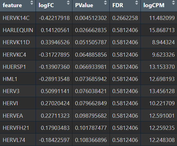
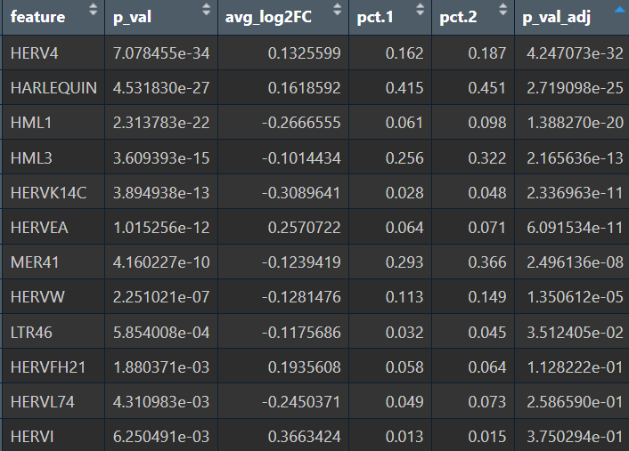
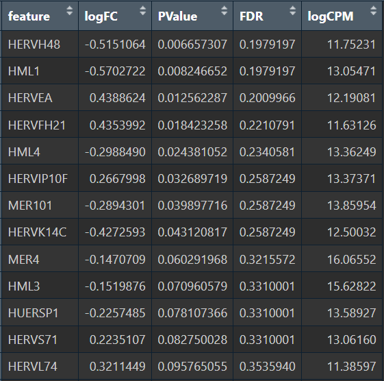
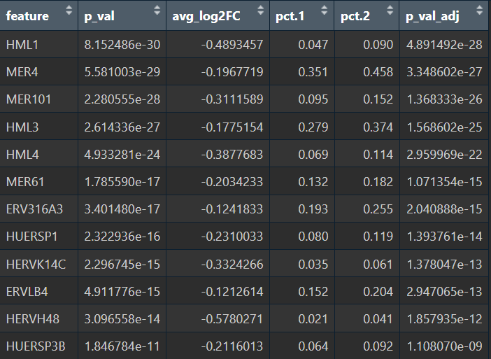
在edgeR过滤特征时,除Endo/Mic这种细胞数本来就少的细胞类型,基本都保留了50个左右的特征
logFC为正值:AD表达更高
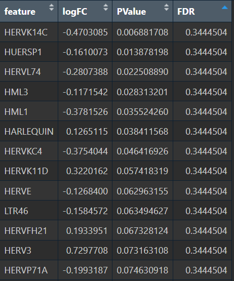
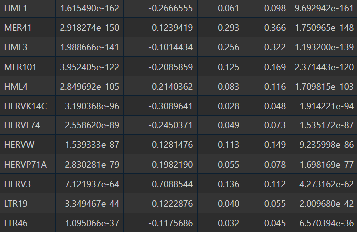
- 全部细胞的5种方法结果:
- edgeR
- Poisson
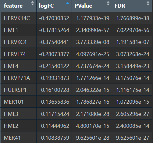
- quasiPoisson
- wilcox
- MAST
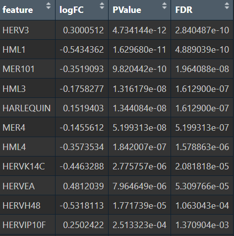
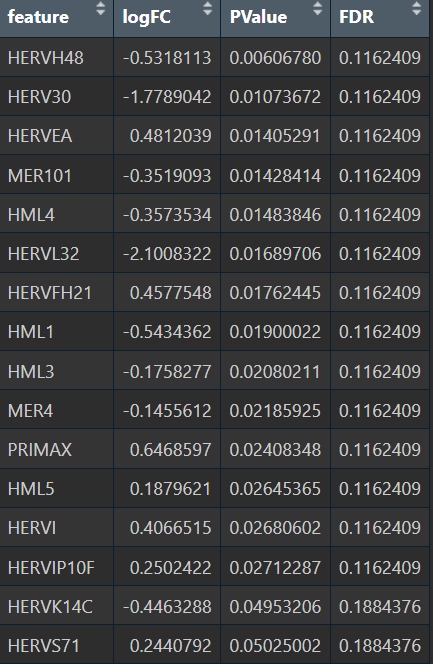
- Astro的5种方法结果:
- edgeR
- Poisson
- quasiPoisson
- wilcox
- MAST
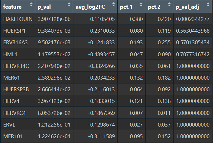
综上,在较大层面上,即使把hERV位点聚合到family水平,信号仍偏弱,并且个体差异/hERV的稀疏性/细胞组成差异会把这个差异冲淡
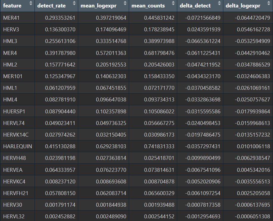
看一下上面结果中比较显著的hERV家族在主要细胞类型中的平均表达分布(差异来自“表达强度”还是“阳性细胞比例/亚群富集”)
astro_sub_col <- "subpop"
# 候选hERV家族
cand <- c(
"HERVK14C","HML1","HERVKC4","HERVL74","HML4","HML3","HML2",
"MER101","MER41","MER4","HUERSP1","HARLEQUIN",
"HERVFH21","HERVEA","HERV3","HERVH48","HERV30","HERVL32"
)
features <- intersect(cand, rownames(seu[[assay_herv]]))
# 计算AD/NC的detect_rate/mean
summarize_family <- function(seu, features, cells_use, herv_assay = assay_herv, group_col = group_col_name, level_name = "ALL") {
md <- seu@meta.data[cells_use, , drop = FALSE]
grp <- as.character(md[[group_col]])
Xc <- GetAssayData(seu, assay = herv_assay, layer = "counts")[features, cells_use, drop = FALSE]
Xd <- GetAssayData(seu, assay = herv_assay, layer = "data")[features, cells_use, drop = FALSE]
out <- lapply(c("NC","AD"), function(g) {
idx <- which(grp == g)
Xc_g <- Xc[, idx, drop = FALSE]
Xd_g <- Xd[, idx, drop = FALSE]
data.frame(
level = level_name,
group = g,
n_cells = length(idx),
feature = features,
detect_rate = Matrix::rowMeans(Xc_g > 0),
mean_logexpr= Matrix::rowMeans(Xd_g),
mean_counts = Matrix::rowMeans(Xc_g),
row.names = NULL,
stringsAsFactors = FALSE
)
})
do.call(rbind, out)
}
# 所有细胞+6个细胞大类+astro聚类
res_all <- summarize_family(seu, features, colnames(seu), level_name = "ALL")
ct <- as.character(seu@meta.data[[celltype_col_name]])
celltypes <- sort(unique(ct))
res_ct <- do.call(rbind, lapply(celltypes, function(k) {
cells_use <- rownames(seu@meta.data)[ct == k]
summarize_family(seu, features, cells_use, level_name = k)
}))
sublab <- as.character(scRNA_astro@meta.data[, astro_sub_col])
sublabs <- sort(unique(sublab))
astro_cells <- rownames(scRNA_astro@meta.data)[T]
res_astro_sub <- do.call(rbind, lapply(sublabs, function(s) {
cells_use <- astro_cells[sublab == s]
summarize_family(scRNA_astro, features, cells_use, level_name = paste0("Astro_", s))
}))
summary_tab <- rbind(res_all, res_ct, res_astro_sub)
summary_tab$delta_detect <- NA_real_
summary_tab$delta_logexpr <- NA_real_
# 给每个level-feature计算AD-NC的差
key <- paste(summary_tab$level, summary_tab$feature, sep = "||")
for (k in unique(key)) {
i <- which(key == k)
if (length(i) != 2) next
if (!all(sort(summary_tab$group[i]) == c("AD","NC"))) next
ad <- i[summary_tab$group[i] == "AD"]
nc <- i[summary_tab$group[i] == "NC"]
summary_tab$delta_detect[i] <- summary_tab$detect_rate[ad] - summary_tab$detect_rate[nc]
summary_tab$delta_logexpr[i] <- summary_tab$mean_logexpr[ad] - summary_tab$mean_logexpr[nc]
}
save(summary_tab, file = "C:\\Users\\17185\\Desktop\\hERV_calc\\GSE157827\\my_data\\0116_2.RData")
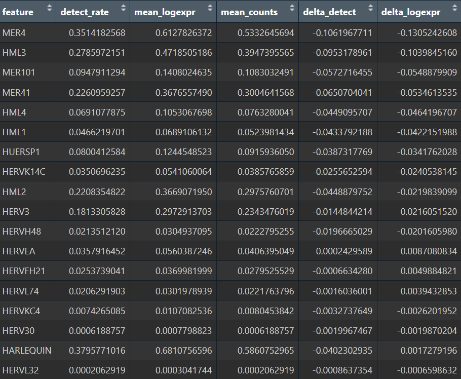
all_res <- summary_tab %>%
filter(level=="ALL", group=="AD") %>%
arrange(-abs(delta_logexpr))
View(all_res)
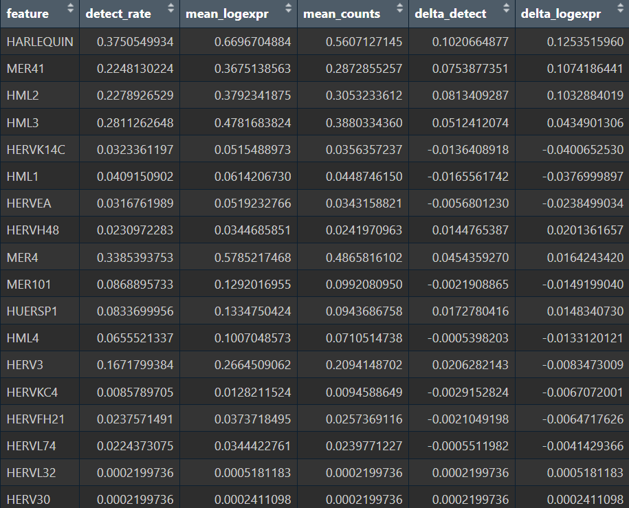
astro_res <- summary_tab %>%
filter(level=="Astro", group=="AD") %>%
arrange(-abs(delta_logexpr))
View(astro_res)
astro_sub_res <- summary_tab %>%
filter(level=="Astro_Up", group=="AD") %>%
arrange(-abs(delta_logexpr))
View(astro_sub_res)
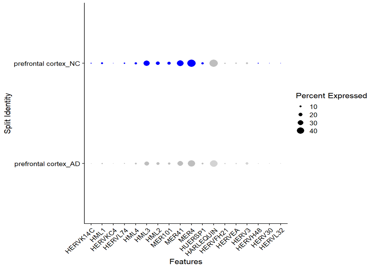
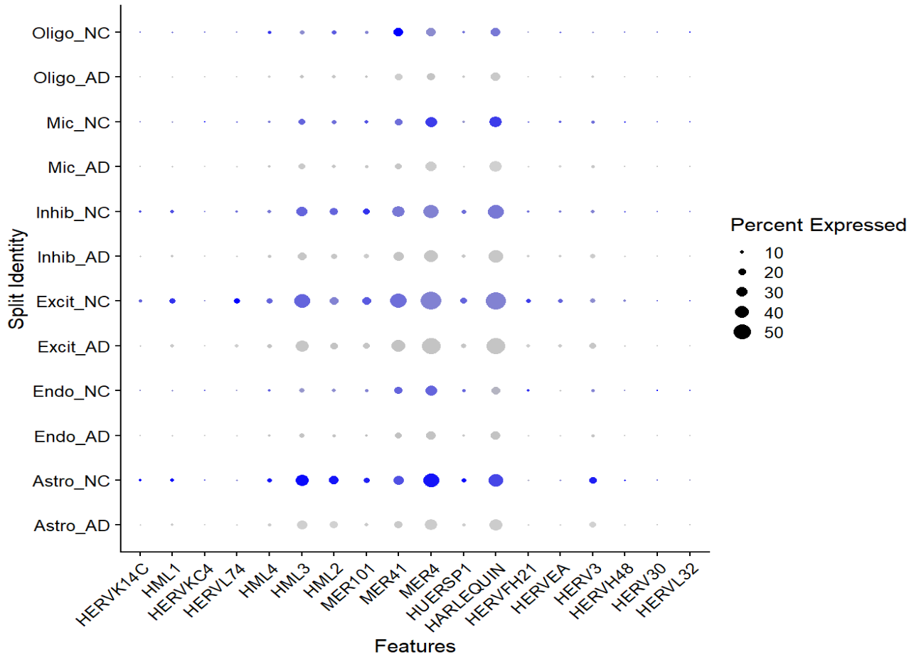
# 所有细胞的hERV家族表达可视化(点大小=percent expressed,颜色=avg exp)
DotPlot(
seu, features = features,
assay = assay_herv,
group.by = "tissue",
split.by = group_col_name
) + RotatedAxis()
# 6个细胞大类
DotPlot(
seu, features = features,
assay = assay_herv,
group.by = celltype_col_name,
split.by = group_col_name
) + RotatedAxis()
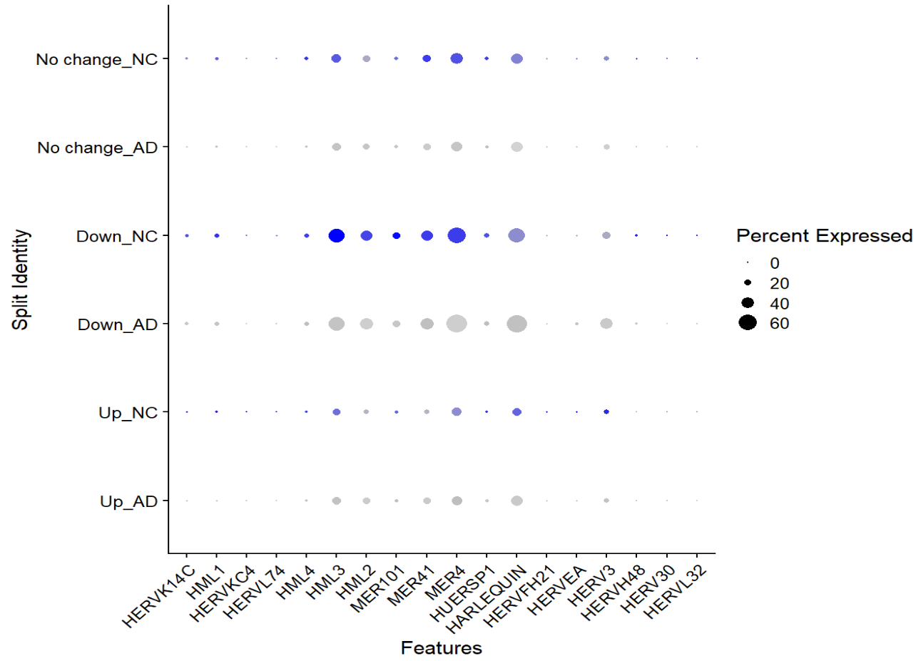
# Astro子群
DotPlot(
scRNA_astro, features = features,
assay = assay_herv,
group.by = astro_sub_col,
split.by = group_col_name
) + RotatedAxis()
-
所有细胞的AD-NC对比
-
astro的hERV表达计量和6个细胞大类的hERV表达图谱
-
Astro细胞按up/down分组,AD_up的hERV表达计量和分组后的hERV表达图谱
再试一试新思路:把AD_Up中的AD细胞与整个astro亚群的NC细胞进行差异分析
assay_use    <- "HERV_family"
celltype_col <- "celltype"
subpop_col   <- "subpop"
group_col    <- "group"
sample_col   <- "orig.ident"
md <- scRNA_astro@meta.data
cells_case <- rownames(md)[md[[celltype_col]] == "Astro" &
                           md[[subpop_col]]   == "Up" &
                           md[[group_col]]    == "AD"]
cells_ctrl <- rownames(md)[md[[celltype_col]] == "Astro" &
                           md[[group_col]]    == "NC"]
cells_use <- union(cells_case, cells_ctrl)
sub <- subset(scRNA_astro, cells = cells_use)
sub$comp <- ifelse(colnames(sub) %in% cells_case, "AD_up_AD", "Astro_NC")
DefaultAssay(sub) <- assay_use
Idents(sub) <- "comp"
# 普通单细胞
de_mast <- FindMarkers(
  sub,
  ident.1 = "AD_up_AD",
  ident.2 = "Astro_NC",
  test.use = "MAST",
  latent.vars = sample_col,
  logfc.threshold = 0,
  min.pct = 0.01
)
de_wilcox <- FindMarkers(
  sub,
  ident.1 = "AD_up_AD",
  ident.2 = "Astro_NC",
  logfc.threshold = 0,
  min.pct = 0.01
)
View(de_mast[order(de_mast$p_val_adj), ])
View(de_wilcox[order(de_mast$p_val_adj), ])
# edgeR
X <- GetAssayData(seu, assay = assay_use, slot = "counts")[, cells_use, drop = FALSE]
samp <- md[cells_use, sample_col]
grp  <- ifelse(cells_use %in% cells_case, "AD_up_AD", "Astro_NC")
M <- sparse.model.matrix(~0 + factor(samp))
colnames(M) <- levels(factor(samp))
pb <- X %*% M
meta_samp <- data.frame(
  sample  = colnames(pb),
  group   = tapply(grp, samp, function(x) unique(x)),
  n_cells = as.integer(table(samp)[colnames(pb)])
)
stopifnot(all(lengths(meta_samp$group) == 1))
meta_samp$group <- factor(unlist(meta_samp$group), levels = c("Astro_NC", "AD_up_AD"))
y <- DGEList(counts = pb, group = meta_samp$group)
keep <- filterByExpr(y, group = meta_samp$group)
y <- y[keep, , keep.lib.sizes = FALSE]
y <- calcNormFactors(y)
design <- model.matrix(~ group, data = meta_samp)
y <- estimateDisp(y, design)
fit <- glmQLFit(y, design)
qlf <- glmQLFTest(fit, coef = "groupAD_up_AD")
de_edger <- topTags(qlf, n = Inf)$table
View(de_edger)
# 保存结果
save(de_mast, de_wilcox, de_edger, file = "C:\\Users\\17185\\Desktop\\hERV_calc\\GSE157827\\my_data\\0117_1.RData")
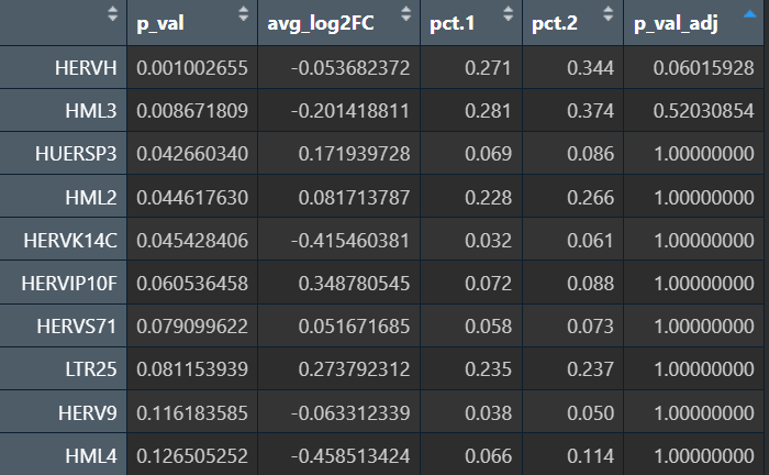
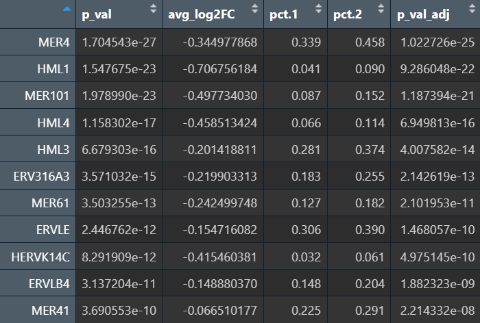
可以看到结果确实更显著了一些。综合上述结果,发现有几个HMLx、MERx表达差异还是挺稳健的,由此可以先确定我们研究的主要hERV家族?
try1
根据讨论时定的方向“有没有哪些细胞类型/亚群的hERV表达有差别”、“根据某些hERV的表达情况来找特殊亚群”,尝试第一个新方向:
- 把几个关键hERV家族统一成一个模块(signature)
- 给每个细胞打分,定义HERV-high/HERV-low(类似于之前AD_up/AD_down的思路?)
- 看它们富集在哪些细胞类型/状态/AD亚群
- 与基因共表达联动
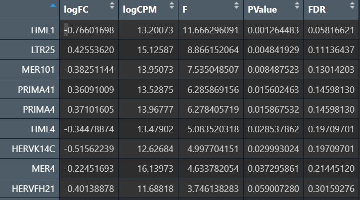
先做一个简单的尝试:就使用上面edgeR的结果,加上我自己判定的比较常见的hERV家族
- sig_up(logFC>0,Up组/AD表达更高):HML5、HML2、HML6、LTR25、LTR19、HERVFH21、HERVFRD、HERVEA、HERV4、HERVIP10F、HERVIP10FH、HERVK11
- sig_down:HML1、HML3、HML4、HERVK14C、HERVH48、HERVE、HERVW、MER101、MER4
sig_up <- c("HML5","HML2","HML6","LTR25","LTR19","HERVFH21","HERVFRD","HERVEA","HERV4","HERVIP10F","HERVIP10FH","HERVK11")
sig_down <- c("HML1","HML3","HML4","HERVK14C","HERVH48","HERVE","HERVW","MER101","MER4")
assay_herv <- "HERV_family"
# 表达量
Xd <- GetAssayData(scRNA_astro, assay = assay_herv, slot = "data")
DefaultAssay(scRNA_astro) <- assay_herv
scRNA_astro$HERVsigUP_expr   <- if (length(sig_up)==0) NA else Matrix::colMeans(Xd[sig_up, , drop=FALSE])
scRNA_astro$HERVsigDOWN_expr <- if (length(sig_down)==0) NA else Matrix::colMeans(Xd[sig_down, , drop=FALSE])
# 检出比例
Xc <- GetAssayData(scRNA_astro, assay = assay_herv, slot = "counts")
scRNA_astro$HERVsigUP_detect <- if (length(sig_up)==0) NA else Matrix::colMeans(Xc[sig_up, , drop=FALSE] > 0)
scRNA_astro$HERVsigDOWN_detect <- if (length(sig_down)==0) NA else Matrix::colMeans(Xc[sig_down, , drop=FALSE] > 0)
VlnPlot(scRNA_astro, features = c("HERVsigDOWN_expr","HERVsigDOWN_detect"), group.by = "subpop", pt.size = 0)
VlnPlot(scRNA_astro, features = c("HERVsigDOWN_expr","HERVsigDOWN_detect"), group.by = "subpop", split.by="group", pt.size = 0)
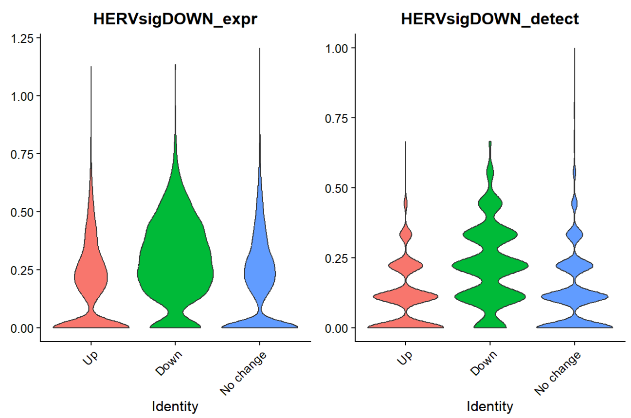
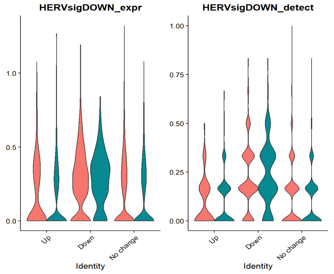
down基因在down组中表达更高,虽然不是特别明显。因为Up基因的FDR普遍较高(FDR<0.2的基因几乎都是down,所以拿down基因定义HERV-high/low状态:
- 在Astro内用detect分位数切HERV-high/low
- 看它是否富集在Down/Up
x <- scRNA_astro$HERVsigDOWN_detect
# 定义HERV-high/low
q_hi <- quantile(x, 0.8, na.rm = TRUE)
q_lo <- quantile(x, 0.2, na.rm = TRUE)
scRNA_astro$HERVclass_sigDOWN <- ifelse(x >= q_hi, "HERV-high",
                           ifelse(x <= q_lo, "HERV-low", "mid"))
table(scRNA_astro$HERVclass_sigDOWN, useNA="ifany")
# 每个subpop里high/low比例
tab_state <- table(scRNA_astro$HERVclass_sigDOWN, scRNA_astro$subpop)
prop.table(tab_state, 2)
> prop.table(tab_state, 2)
                   Up      Down No change
  HERV-high 0.2588884 0.6128544 0.3020725
  HERV-low  0.3996731 0.1209830 0.3711555
  mid       0.3414385 0.2661626 0.3267720
> tab_state
              Up Down No change
  HERV-high 1267 1621      3192
  HERV-low  1956  320      3922
  mid       1671  704      3453
整体来说符合预期——AD_down中有较多的down基因表达高(HERV-high)的细胞,AD_up中较少,No change介于两者之间,说明”sigDOWN”定义的high和low确实能够对应不同状态。结合我前面画的小提琴图,可以看到在AD-NC的层面,”sigDOWN”差别不大,所以这里的信号主要来自AD_down/up的状态差异,而不是“疾病主效应”(AD的差异基因/差异hERV不稳健很正常,更值得做的是“状态/亚群层面的解释”)
与基因结合分析:
- 在astro内的HERV-high与HERV-low中做基因差异
- 做GO/通路富集
- 看这些基因模块与Up/Down的关系
DefaultAssay(scRNA_astro) <- "HERV_family"
seuA <- subset(scRNA_astro, subset = HERVclass_sigDOWN %in% c("HERV-high","HERV-low"))
DefaultAssay(seuA) <- "RNA"
Idents(seuA) <- "HERVclass_sigDOWN"
de_hervHL_res <- FindMarkers(
  seuA,
  ident.1 = "HERV-high",
  ident.2 = "HERV-low",
  # test.use = "MAST",
  # latent.vars = c("orig.ident"),
)
de_hervHL <- de_hervHL_res %>%
  rownames_to_column("gene") %>%
  filter(p_val_adj < 0.05, abs(avg_log2FC) >= 0.25) %>%
  filter(pct.1 >= 0.1 | pct.2 >= 0.1) %>%
  filter(!grepl("^(ENSG|MT-|LINC-)|(AC|AL)[0-9]", gene))
up_genes <- (filter(de_hervHL, avg_log2FC > 0))$gene  # HERV-high更高表达
down_genes <- (filter(de_hervHL, avg_log2FC < 0))$gene
# 背景基因:Astro里检测到过的基因
expr_counts <- GetAssayData(seuA, assay = "RNA", slot = "counts")
bg <- rownames(expr_counts)[Matrix::rowSums(expr_counts > 0) >= 10]
ego_up <- enrichGO(
gene = up_genes,
universe = bg,
OrgDb = org.Hs.eg.db,
keyType = "SYMBOL",
ont = "BP",
pAdjustMethod = "BH",
qvalueCutoff = 1,
pvalueCutoff = 1,
readable = TRUE
)
ego_down <- enrichGO(
gene = down_genes,
universe = bg,
OrgDb = org.Hs.eg.db,
keyType = "SYMBOL",
ont = "BP",
pAdjustMethod = "BH",
qvalueCutoff = 1,
pvalueCutoff = 1,
readable = TRUE
)
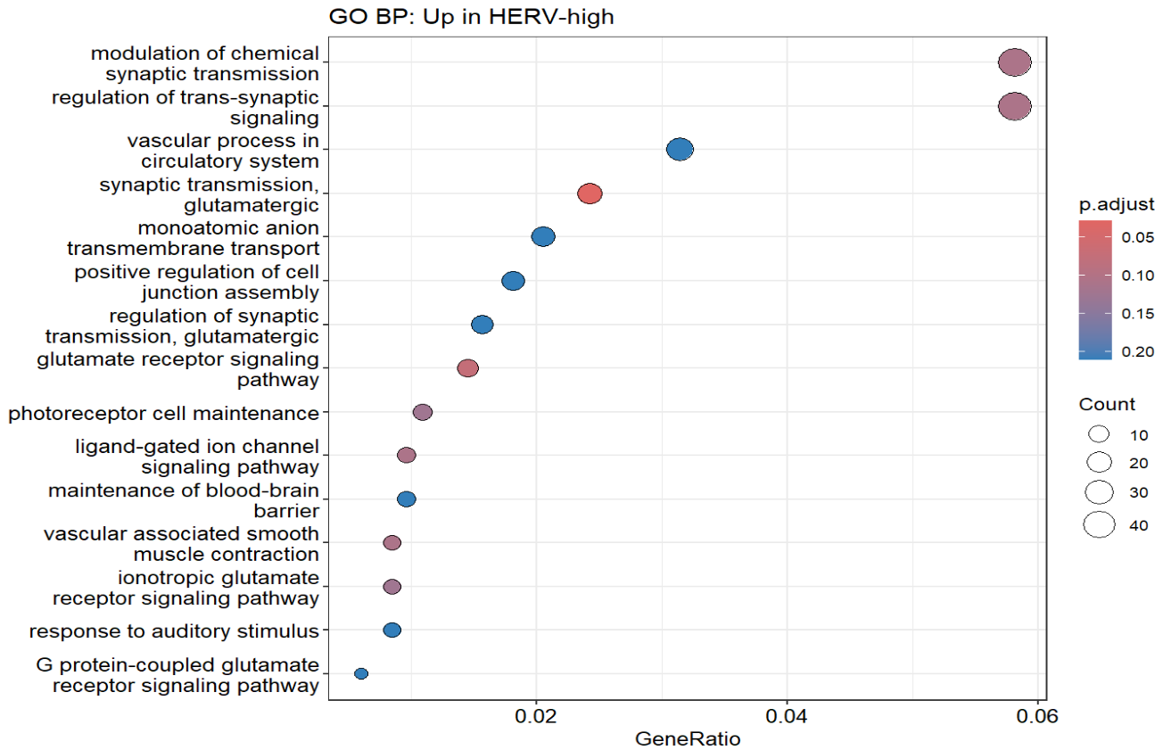
dotplot(ego_up, showCategory = 15) + ggtitle("GO BP: Up in HERV-high")
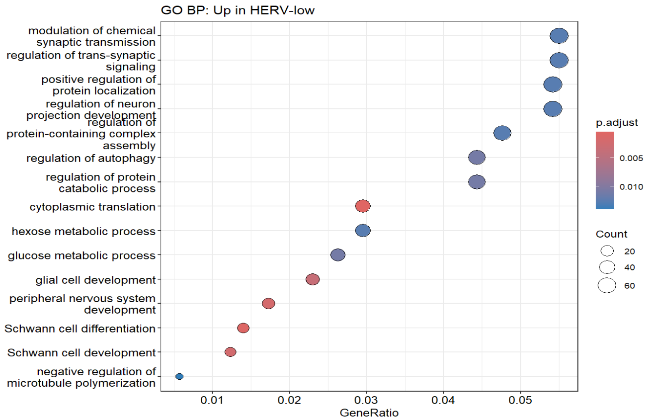
dotplot(ego_down, showCategory = 15) + ggtitle("GO BP: Up in HERV-low")
Xd <- GetAssayData(seuA, assay="RNA", slot="data")
up_genes2   <- intersect(up_genes, rownames(Xd))
down_genes2 <- intersect(down_genes, rownames(Xd))
seuA$GeneSig_HERVhigh_expr <- Matrix::colMeans(Xd[up_genes2, , drop=FALSE])
seuA$GeneSig_HERVlow_expr  <- Matrix::colMeans(Xd[down_genes2, , drop=FALSE])
# 这些基因在Up/Down/No change上是否有梯度
VlnPlot(seuA,
        features = c("GeneSig_HERVhigh_expr","GeneSig_HERVlow_expr"),
        group.by = "subpop",
        split.by = "group",
        pt.size = 0)
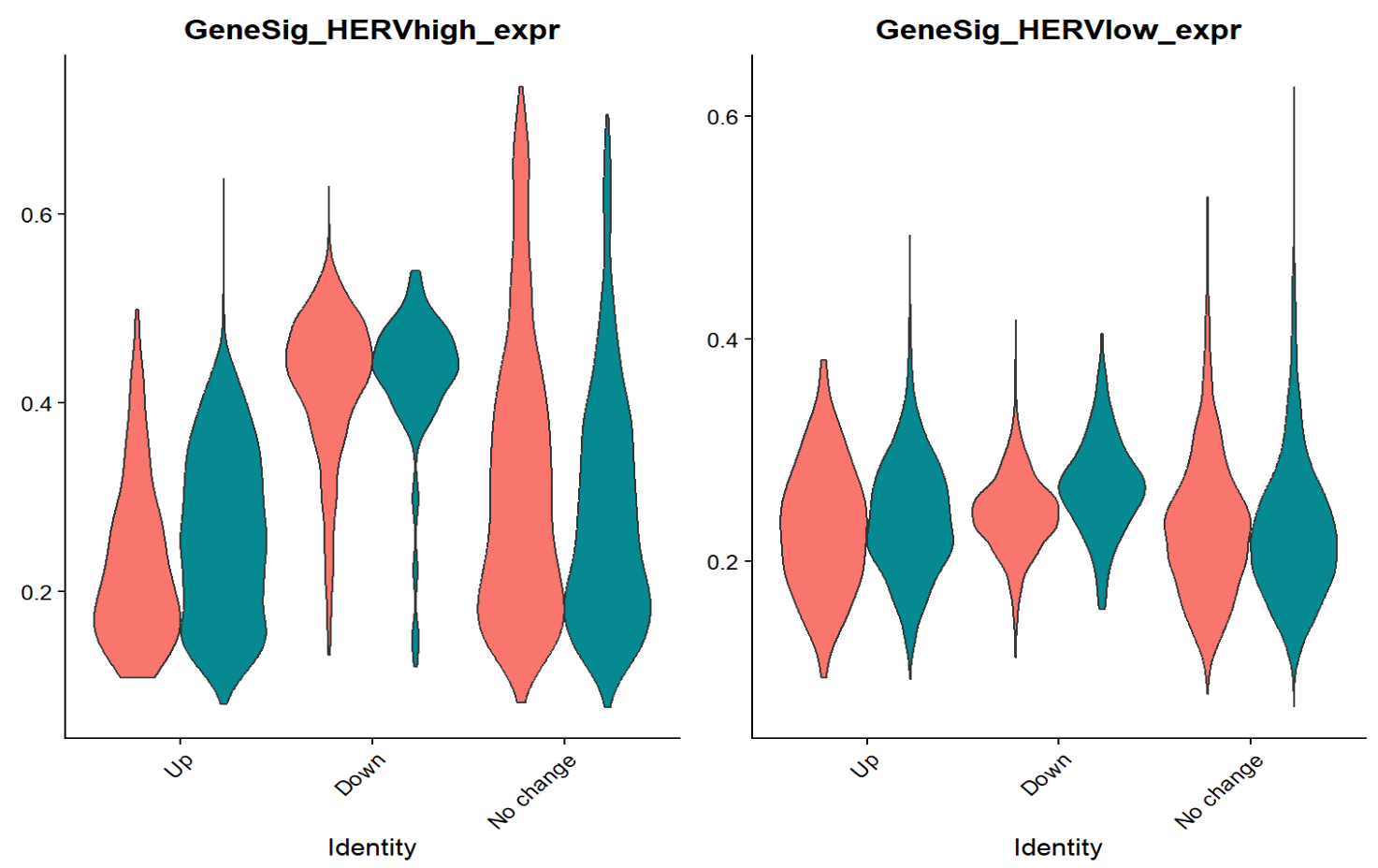
通过富集结果,可以看出HERV-high与HERV-low的差异基因确实是与神经系统有关(虽然神经系统的GO条目占比并不多,不过联想到之前跟教程走的结果,其实还可以接受)
GeneSig_HERVhigh_expr这个分数在Down组最高(某些ERV/LTR的检出率高),同时一些神经系统相关的基因上调(这套基因程序在Down状态最强)- 我之后又使用了edgeR做了样本级的差异分析,结果类似
附上GPT对这段的解读:
- 用ERV/hERV的家族signature定义了新的“ERV-activity状态”
- 该状态与astro的Up/Down强相关
- 该状态对应一组基因表达程序(炎症/应激/IFN等)
- AD的作用更多体现在状态比例/调制,而非稳定主效应
这就是一个简易版的基因共表达?
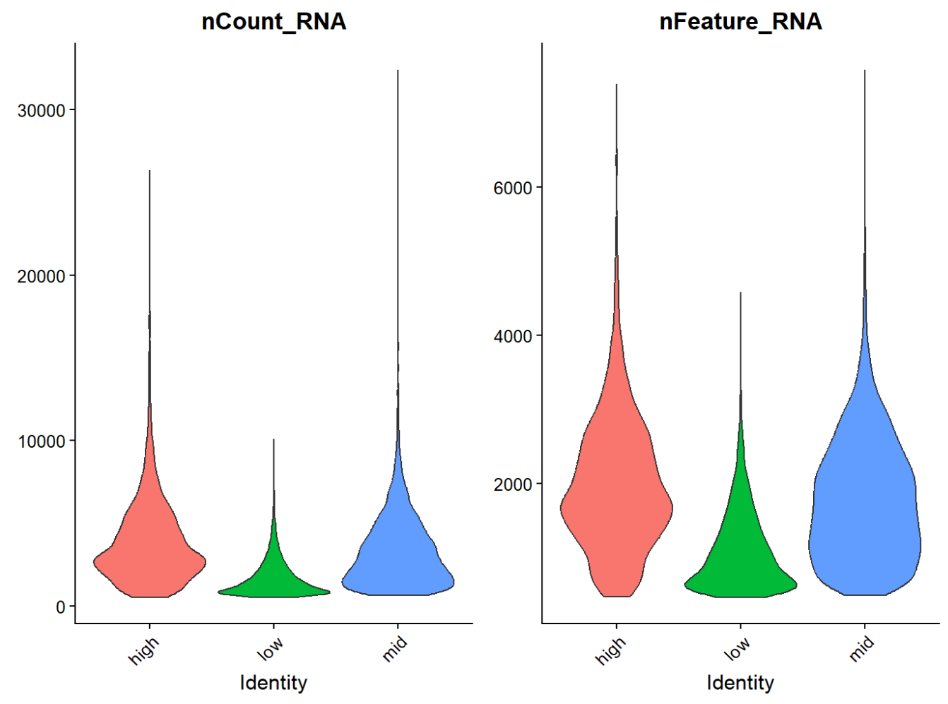
之后我又看了HERV-high与HERV-low的nCount/Feature_RNA情况:
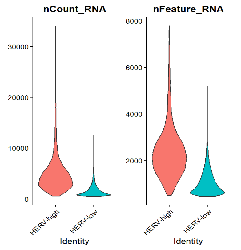
感觉这个HERV-high/low的划分就有些诡异(受到测序深度/复杂度影响很大)
try2
能不能在try1的基础上简化一些?
- 不分那么多的细胞类群(HERV-high、HERV-low这种),就使用6个细胞大类,以及Astro和Oligo的子聚类亚群
- 找某个或某几个关键hERV家族,看其在细胞群体中的表达差异
- 这个差异是否能定义某个亚群(根据hERV家族而不是普通基因划分亚群?)
- 这个差异与哪些基因有关(hERV与基因的共表达),是否有“某个基因的表达量与某个hERV家族的表达相关”
首先为了提高分析的针对性,我用GPT分析了差异表达分析的结果(5种方法在所有细胞和astro细胞中 AD-NC的差异)
- 最核心的几个:
- HML1 / HML3 / HML4 / HERVK14C:基本都属于HERV-K谱系,常被拿来讨论潜在转录/蛋白表达与疾病相关性;同时检出率也不算太低
- MER101:MER是ERV/LTR衍生的重复元件家族,可用于说明“ERV/LTR的转录/调控状态变化”
- HERVH48:HERV-H48(可能不属于HERV-H大类,使用的命名体系不同?)
- 可选:
- MER41:提供转录因子结合位点、参与干扰素应答调控网络,可用于说明“AD炎症/免疫环境变化”
- HERV-W:HERV-W家族相关的env(Syncytin-1)也有一些相关研究
- HERVEA:HERV-E家族在不同组织/疾病里经常被讨论(尤其肿瘤方向较多)
- HARLEQUIN:虽然相关研究较少,但在差异分析结果中频繁出现
- 上述hERV家族,好像只有HERVEA是AD上调,其它都是下调
先画几张“单family分布图”直观看
assay_herv <- "HERV_family"
assay_rna  <- "RNA"
astro_sub_col <- "sle_reso"
DefaultAssay(seu) <- assay_herv
DefaultAssay(scRNA_astro) <- assay_herv
panel <- c("HML1","HML3","HML4","HERVK14C","MER101","HERVH48",
             "MER41","HERVW","HARLEQUIN","HERVEA")
to_plot <- c("HML1","HERVEA","HERVH48","MER101")
# UMAP上看表达
FeaturePlot(seu, features = to_plot, reduction = "umap", order = TRUE)
# Astro子群里的分布
FeaturePlot(scRNA_astro, features = to_plot, reduction = "umap", order = TRUE)
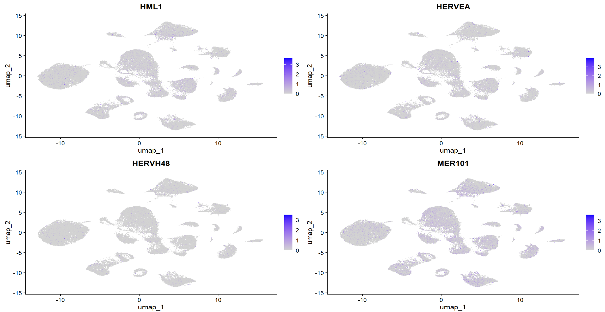
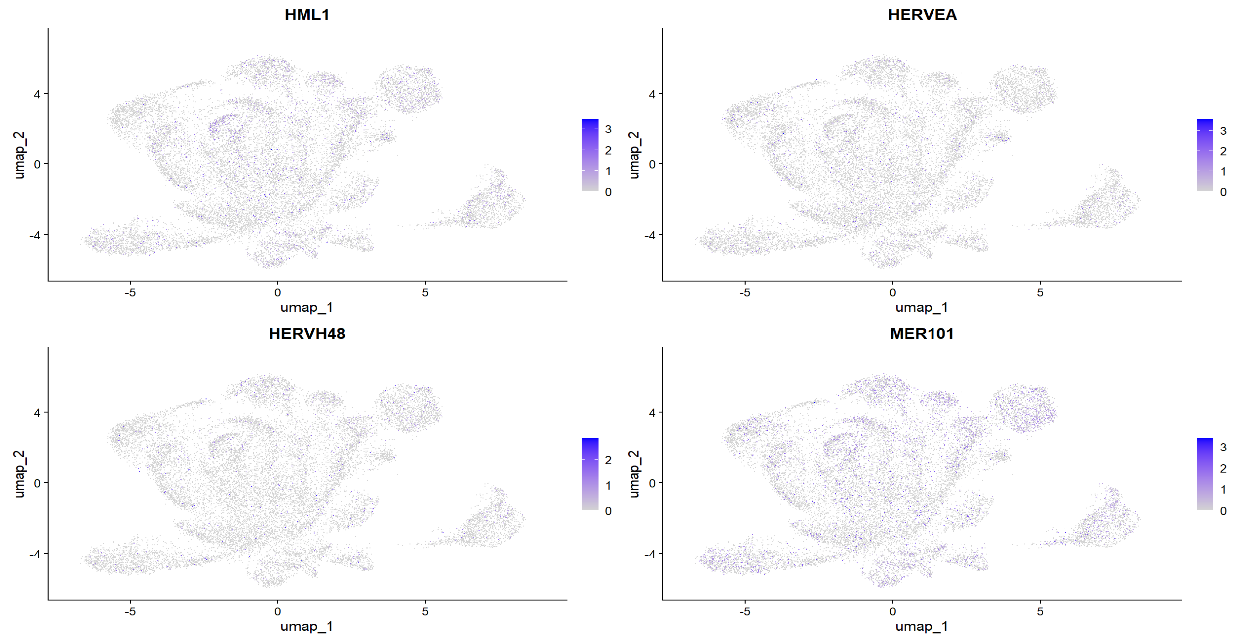
可以看到,即使把hERV聚合到family级别,总体仍比较稀疏,对于某一家族,并不是大多数细胞都有表达
计算panel分数:expr_score/detect_score
# 计算候选hERV家族的分数
Xd <- GetAssayData(seu, assay = assay_herv, slot = "data")[panel, , drop = FALSE]
Xc <- GetAssayData(seu, assay = assay_herv, slot = "counts")[panel, , drop = FALSE]
seu$herv_expr_score <- Matrix::colMeans(Xd)
seu$herv_detect_score <- Matrix::colMeans(Xc > 0)
Xd <- GetAssayData(scRNA_astro, assay = assay_herv, slot = "data")[panel, , drop = FALSE]
Xc <- GetAssayData(scRNA_astro, assay = assay_herv, slot = "counts")[panel, , drop = FALSE]
scRNA_astro$herv_expr_score <- Matrix::colMeans(Xd)
scRNA_astro$herv_detect_score <- Matrix::colMeans(Xc > 0)
# 在astro内把候选hERV家族分成up和down,分别计算分数
# 因为是根据astro的差异表达结果分的,所以只在astro内计算
up_set <- c("HARLEQUIN","HERVEA")
down_set <- c("HML1","HML3","HML4","HERVK14C","MER101","HERVH48","MER41","HERVW")
scRNA_astro$herv_up_expr <- Matrix::colMeans(Xd[up_set, , drop=FALSE])
scRNA_astro$herv_up_detect <- Matrix::colMeans(Xc[up_set, , drop=FALSE] > 0)
scRNA_astro$herv_down_expr <- Matrix::colMeans(Xd[down_set, , drop=FALSE])
scRNA_astro$herv_down_detect <- Matrix::colMeans(Xc[down_set, , drop=FALSE] > 0)
# 在Astro内按分位选出hERV-high/low
make_state <- function(x, q_lo = 0.2, q_hi = 0.8) {
  lo <- quantile(x, q_lo, na.rm = TRUE)
  hi <- quantile(x, q_hi, na.rm = TRUE)
  ifelse(x >= hi, "high", ifelse(x <= lo, "low", "mid"))
}
metaA <- scRNA_astro@meta.data
metaA$herv_state <- make_state(metaA$herv_detect_score)
# 看它是否富集在某些Astro子群
tab1 <- prop.table(table(metaA$herv_state, metaA[[astro_sub_col]]), 2)
# 看AD/NC是否富集
tab2 <- prop.table(table(metaA$herv_state, metaA$group), 2)
df_sample <- metaA %>%
  group_by(orig.ident, group) %>%
  summarise(frac_high = mean(herv_state=="high"),
            frac_low  = mean(herv_state=="low"),
            mean_det  = mean(herv_detect_score),
            .groups="drop")
wilcox.test(frac_high ~ group, data=df_sample)
wilcox.test(frac_low  ~ group, data=df_sample)
wilcox.test(mean_det  ~ group, data=df_sample)
> print(tab1)
               a1        a10        a11        a12
  high 0.16137194 0.52020202 0.50948509 0.03973510
  low  0.29828507 0.05808081 0.04607046 0.47019868
  mid  0.54034299 0.42171717 0.44444444 0.49006623
               a2         a3         a4         a5
  high 0.09337094 0.07827059 0.40797872 0.17536141
  low  0.39576869 0.37644428 0.12925532 0.24827153
  mid  0.51086037 0.54528513 0.46276596 0.57636706
               a6         a7         a8         a9
  high 0.30274510 0.41120000 0.08191489 0.36034115
  low  0.21176471 0.16080000 0.40212766 0.08528785
  mid  0.48549020 0.42800000 0.51595745 0.55437100
> print(tab2)
              NC        AD
  high 0.2675068 0.1502837
  low  0.2491975 0.3110882
  mid  0.4832957 0.5386282

data:  frac_high by group
W = 69, p-value = 0.31
data:  frac_low by group
W = 44, p-value = 0.5079
data:  mean_det by group
W = 68, p-value = 0.3451
计算6大细胞类型和astro子群的hERV表达分数和检出率
meta <- seu@meta.data %>%
mutate(cell = rownames(seu@meta.data)) %>%
dplyr::select(cell, orig.ident, group, celltype,
herv_expr_score, herv_detect_score)
# 6大细胞类型在样本层面计算均值
pb_celltype <- meta %>%
group_by(orig.ident, group, celltype) %>%
summarise(n_cells = n(),
detect_frac = mean(herv_detect_score),
mean_expr = mean(herv_expr_score),
.groups = "drop")
# 每个细胞类型里AD-NC
test_celltype <- pb_celltype %>%
group_by(celltype) %>%
summarise(p_detect = tryCatch(wilcox.test(detect_frac ~ group)$p.value, error=function(e) NA_real_),
p_expr = tryCatch(wilcox.test(mean_expr ~ group)$p.value, error=function(e) NA_real_),
.groups="drop")
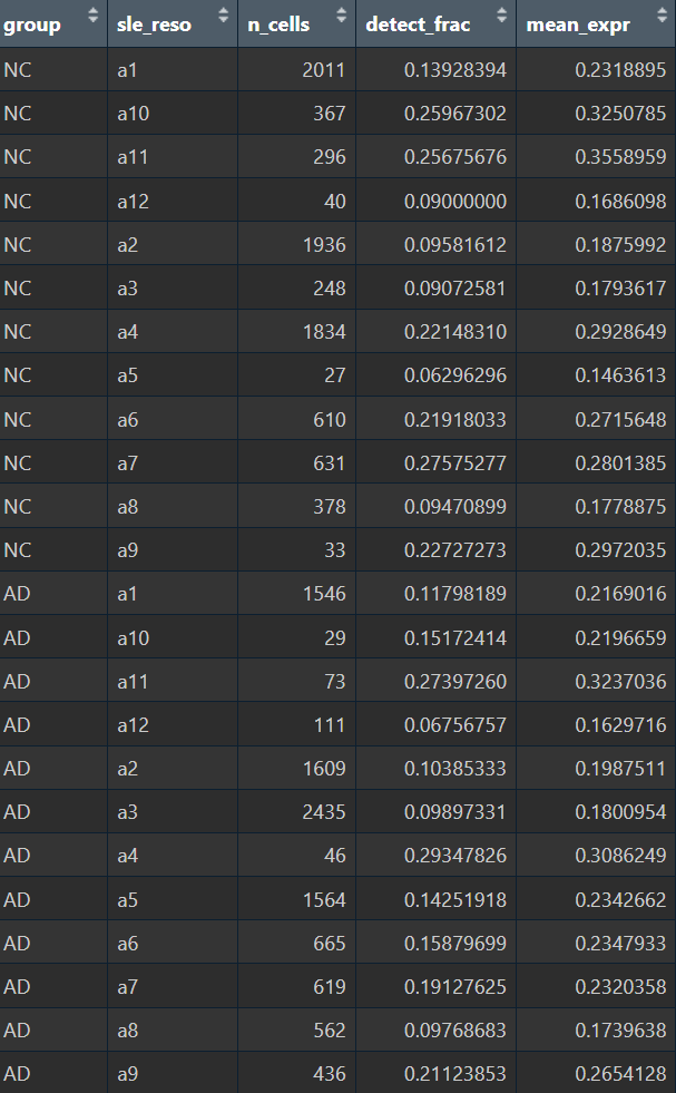
# Astro子群
pb_astro_sub <- scRNA_astro@meta.data %>%
group_by(group, .data[[astro_sub_col]]) %>%
summarise(n_cells = n(),
detect_frac = mean(herv_detect_score),
mean_expr = mean(herv_expr_score),
.groups="drop")
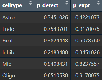
- 在每个细胞类型中,如果按上面选出的这些hERV家族计算分数,AD和NC的分数差异仍不明显,说明选出的hERV家族的表达情况在各细胞类型中并不一致
- 结合tab1/2,在astro内部,不同亚群的检出率和表达量差异较大,说明这种方法计算得到的hERV分数更像是在刻画Astro内部的“hERV活跃度状态”,而不是纯AD效应
- astro各亚群的high/low比例显著不同,说明这个分数确实能“定义一类Astro状态”,但不能稳健地区分AD-NC(AD-NC差异主要来自子群比例改变)
上面都是样本层面看AD-NC的hERV分数差异,试一试细胞层面
meta <- seu@meta.data %>%
mutate(
group = factor(group, levels = c("NC","AD")),
celltype = factor(celltype, levels = c("Astro","Endo","Excit","Inhib","Mic","Oligo"))
) %>%
filter(!is.na(herv_expr_score), !is.na(group), !is.na(orig.ident), !is.na(celltype))
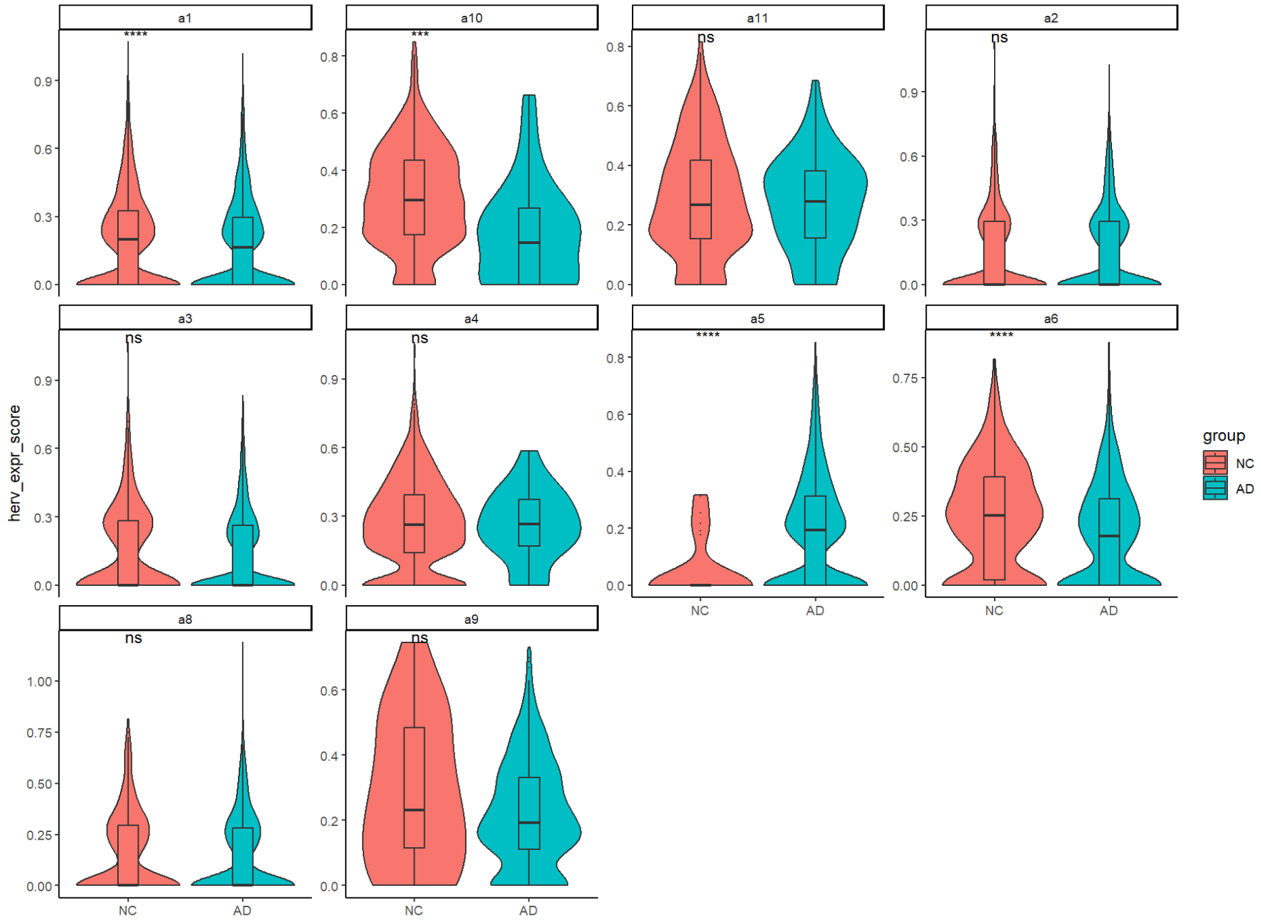
# 每种细胞类型,AD/NC的分数分布
ggplot(meta, aes(x = celltype, y = herv_expr_score, fill = group)) +
geom_violin(scale = "width", trim = TRUE, position = position_dodge(width = 0.8)) +
geom_boxplot(width = 0.12, outlier.size = 0.2, position = position_dodge(width = 0.8)) +
theme_classic() +
ylab("herv_expr_score") + xlab(NULL)
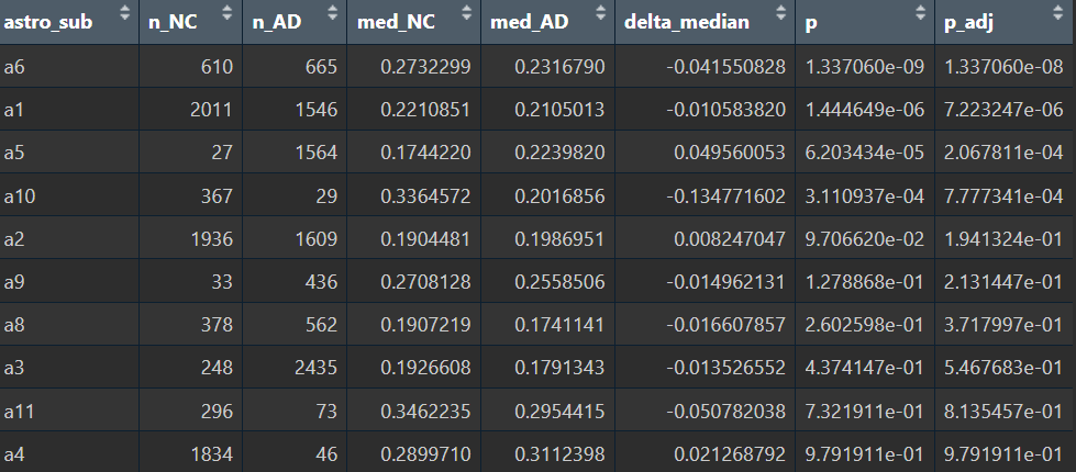
# 算p值
res_cell_wilcox <- meta %>%
group_by(celltype) %>%
summarise(
n_NC = sum(group=="NC"),
n_AD = sum(group=="AD"),
med_NC = median(herv_expr_score[group=="NC"]),
med_AD = median(herv_expr_score[group=="AD"]),
delta_median = med_AD - med_NC,
p = wilcox.test(herv_expr_score ~ group)$p.value,
.groups = "drop"
) %>%
mutate(p_adj = p.adjust(p, method = "BH")) %>%
arrange(p_adj)
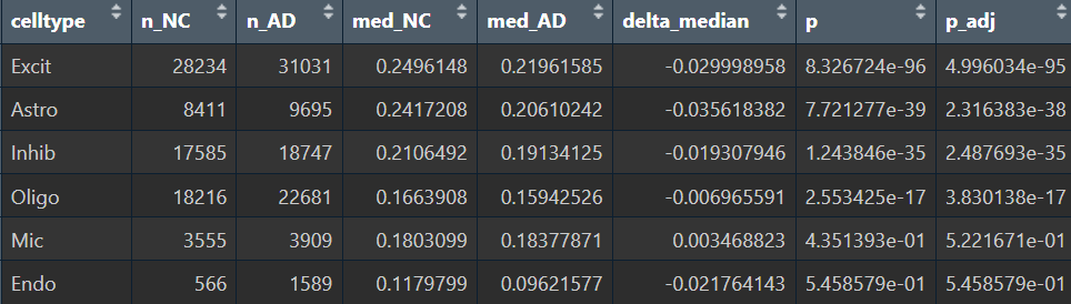
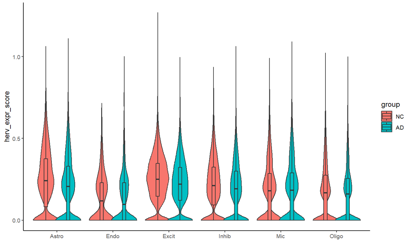
在几个较大细胞类别里还是比较显著的
看我们的hERV分数定义的astro子群
# 看一下样本的平均分数分布(在astro的各亚群内)
pb <- metaA %>%
group_by(orig.ident, group, sle_reso) %>%
summarise(detect_frac = mean(herv_detect_score),
mean_expr = mean(herv_expr_score),
n_cells = n(),
.groups="drop")
sub_rank <- pb %>%
group_by(sle_reso) %>%
summarise(detect_frac = mean(detect_frac),
mean_expr = mean(mean_expr),
.groups="drop") %>%
arrange(desc(detect_frac))
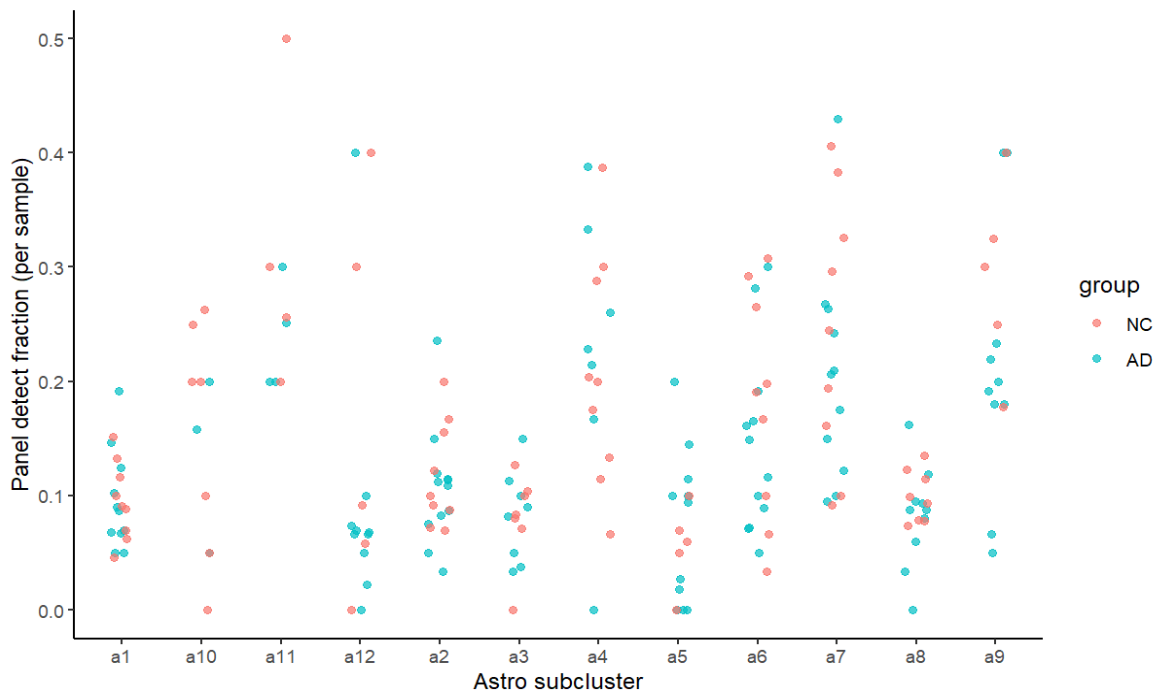
ggplot(pb, aes(x = sle_reso, y = detect_frac, color = group)) +
geom_point(position = position_jitter(width = 0.15), alpha = 0.7) +
theme_classic() +
labs(y="Panel detect fraction (per sample)", x="Astro subcluster")
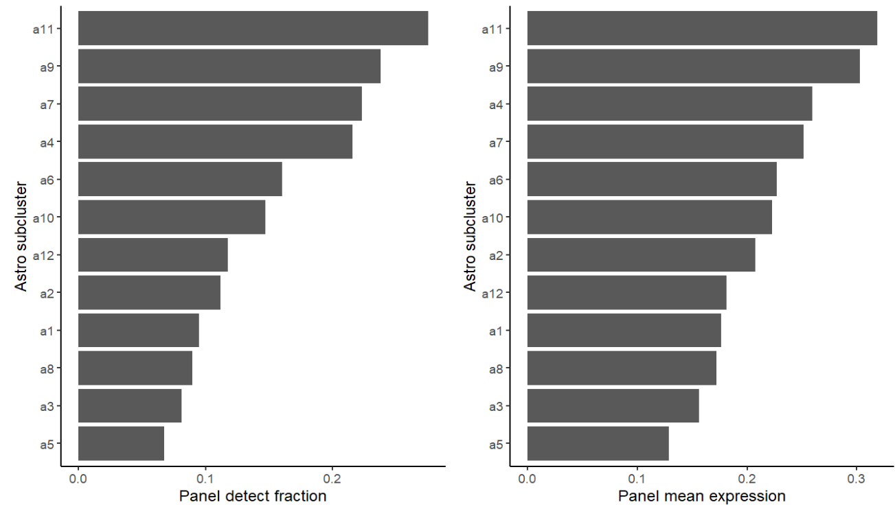
ggplot(sub_rank, aes(x=reorder(sle_reso, detect_frac), y=detect_frac)) +
geom_col() + coord_flip() + theme_classic() +
labs(x="Astro subcluster", y="Panel detect fraction") | ggplot(sub_rank, aes(x=reorder(sle_reso, mean_expr), y=mean_expr)) +
geom_col() + coord_flip() + theme_classic() +
labs(x="Astro subcluster", y="Panel mean expression")
在之前的try1中,在找astro内部亚群的差异基因时,GPT多次提醒我很多差异基因都富集到了突触这类神经元相关的功能上,说astro不会表达这么多神经元相关基因,可能要剔除一些“像神经元”的亚群
DefaultAssay(scRNA_astro) <- "RNA"
Idents(scRNA_astro) <- "sle_reso"
astro_mk <- c("AQP4","GFAP","SLC1A2","SLC1A3","ALDH1L1","CLU")
neuro_mk <- c("RBFOX3","SNAP25","SYT1","SLC17A7","GAD1","GAD2")
DotPlot(scRNA_astro, features = c(astro_mk, neuro_mk)) + RotatedAxis()
VlnPlot(scRNA_astro, features=c("nFeature_RNA","nCount_RNA","percent_mito"), group.by="sle_reso", pt.size=0)
# 改astro
scRNA_astro_clean <- subset(scRNA_astro, subset = sle_reso != "a7")
scRNA_astro_clean <- subset(scRNA_astro_clean, subset = sle_reso != "a12")
saveRDS(
  scRNA_astro_clean,
  file = "C:\\Users\\17185\\Desktop\\hERV_calc\\GSE157827\\my_data\\GSE157827_astro_clean.rds",
  compress = "xz"
)
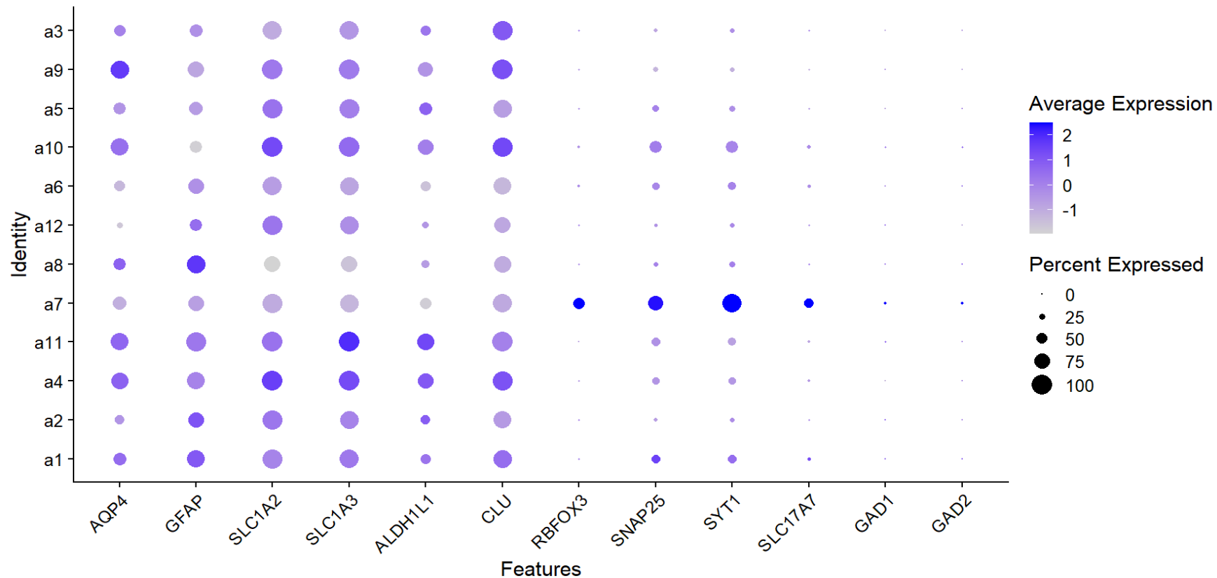
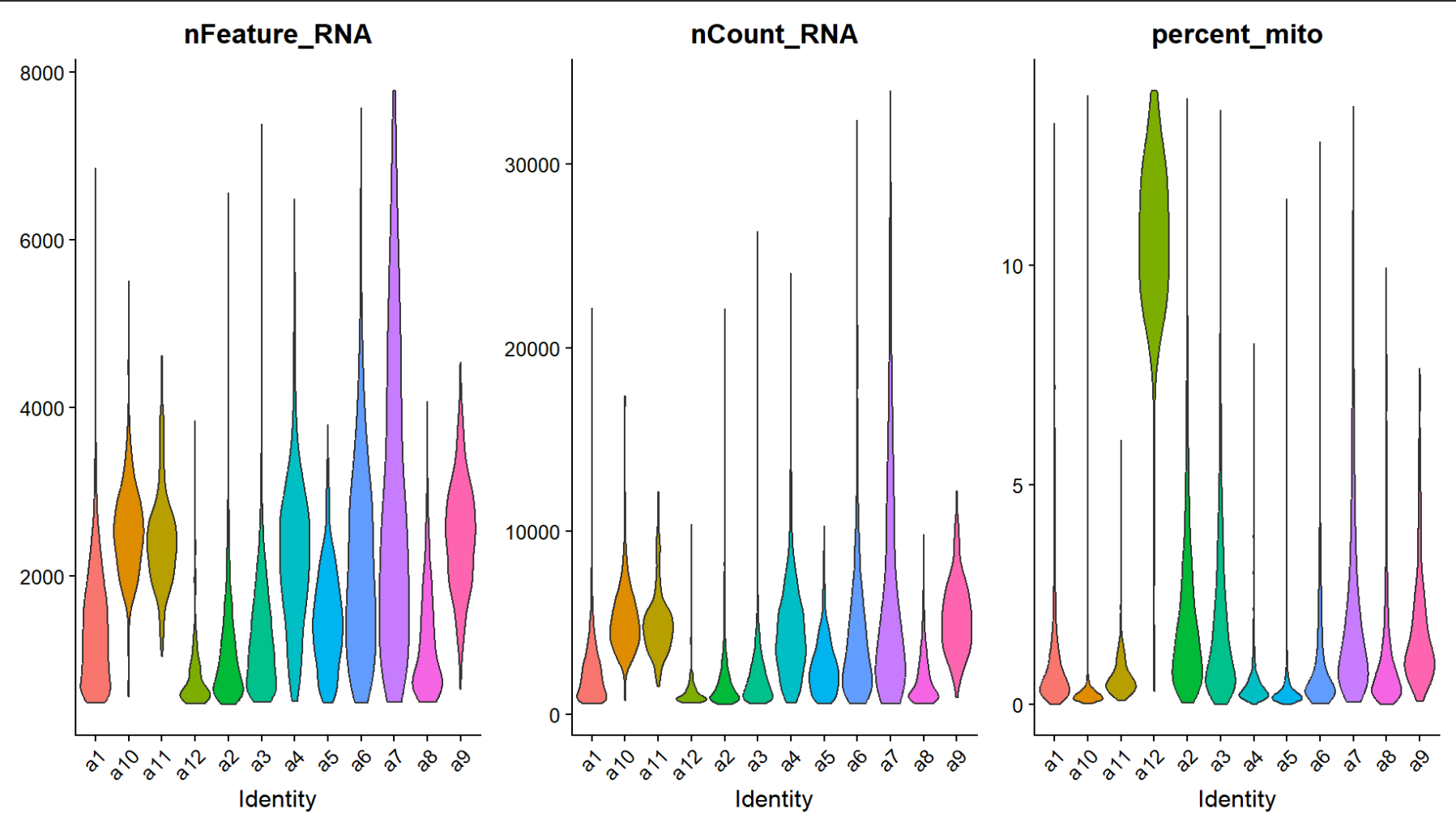
似乎a7和a12是异常的astro细胞,过滤
在astro内的hERV-gene共表达
- 根据subrank的排名,选出HERV-high端(a11/a9/a7/a4)和HERV-low端(a3/a5/a8/a1)
- 看这两端在基因表达上的差别(FindMarkers)
- hERV-gene共表达:哪些基因和“hERV状态轴”同步变化
# 取出HERV-high和HERV-low的细胞
astro_sub_col <- "sle_reso"
high_sub <- c("a11","a9","a4")
low_sub <- c("a5","a3","a8","a1")
scRNA_astro$HERV_state_sub <- ifelse(scRNA_astro[[astro_sub_col]][,1] %in% high_sub, "HERV_high_sub",
ifelse(scRNA_astro[[astro_sub_col]][,1] %in% low_sub, "HERV_low_sub", NA))
scRNA_astro2 <- subset(scRNA_astro, subset = HERV_state_sub %in% c("HERV_high_sub","HERV_low_sub"))
Idents(scRNA_astro2) <- "HERV_state_sub"
# 两组的基因差异
DefaultAssay(scRNA_astro2) <- "RNA"
deg <- FindMarkers(
scRNA_astro2,
ident.1 = "HERV_high_sub",
ident.2 = "HERV_low_sub",
test.use = "MAST",
latent.vars = c("orig.ident", "nCount_RNA", "percent_mito"),
logfc.threshold = 0.1,
min.pct = 0.05
)
deg <- deg %>%
tibble::rownames_to_column("gene") %>%
arrange(p_val_adj) %>%
filter(!grepl("^(ENSG|MT-|LINC)|^(AC|AL)[0-9]", gene))
save(deg, file = "C:\\Users\\17185\\Desktop\\hERV_calc\\GSE157827\\my_data\\0123_1.RData")
# GO分析
deg <- deg %>%
filter(p_val_adj<0.05)
genes_high_up <- deg %>% filter(avg_log2FC > 0) %>% pull(gene) %>% unique()
genes_low_up <- deg %>% filter(avg_log2FC < 0) %>% pull(gene) %>% unique()
DefaultAssay(scRNA_astro_clean) <- "RNA"
expr_counts <- GetAssayData(scRNA_astro_clean, slot = "counts")
universe <- rownames(expr_counts)[Matrix::rowSums(expr_counts > 0) >= 10]
ego_high <- enrichGO(
gene = genes_high_up,
universe = universe,
OrgDb = org.Hs.eg.db,
keyType = "SYMBOL",
ont = "BP",
pAdjustMethod = "BH",
pvalueCutoff = 0.05,
qvalueCutoff = 0.2,
readable = TRUE
)
ego_low <- enrichGO(
gene = genes_low_up,
universe = universe,
OrgDb = org.Hs.eg.db,
keyType = "SYMBOL",
ont = "BP",
pAdjustMethod = "BH",
pvalueCutoff = 0.05,
qvalueCutoff = 0.2,
readable = TRUE
)
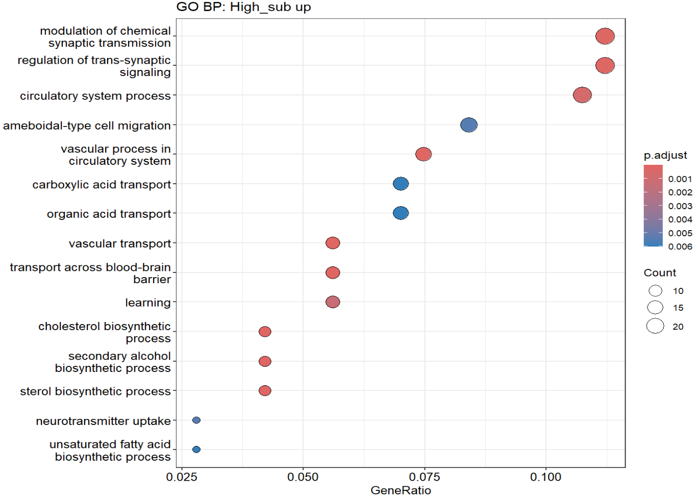
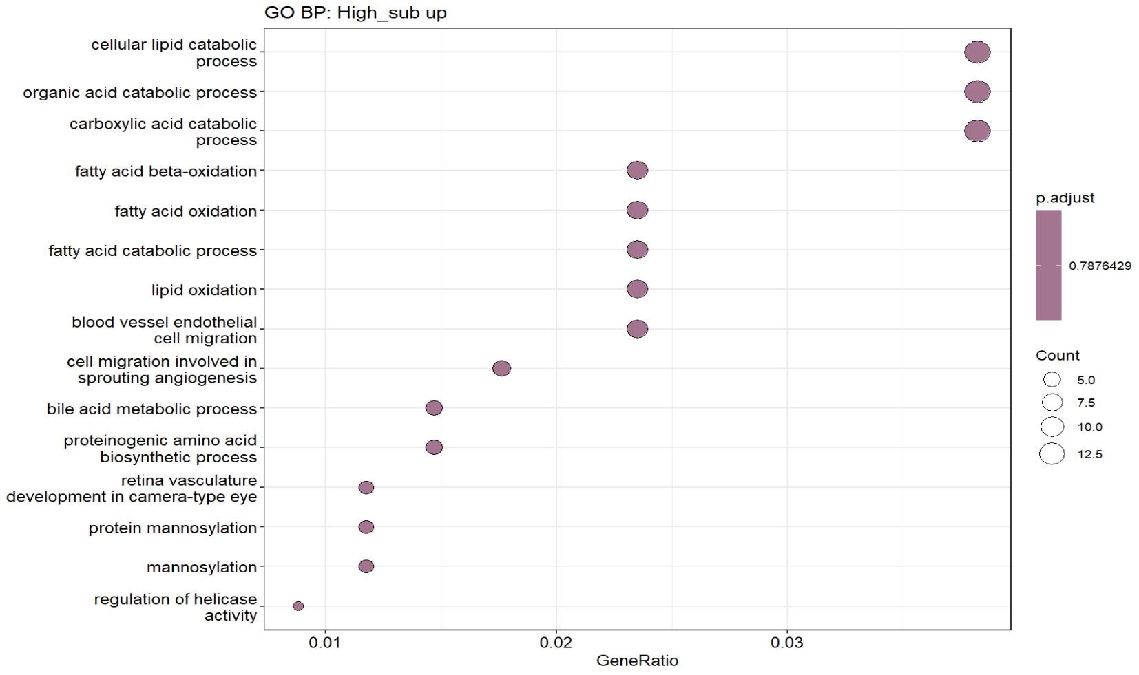
dotplot(ego_high, showCategory = 15) + ggplot2::ggtitle("GO BP: High_sub up")
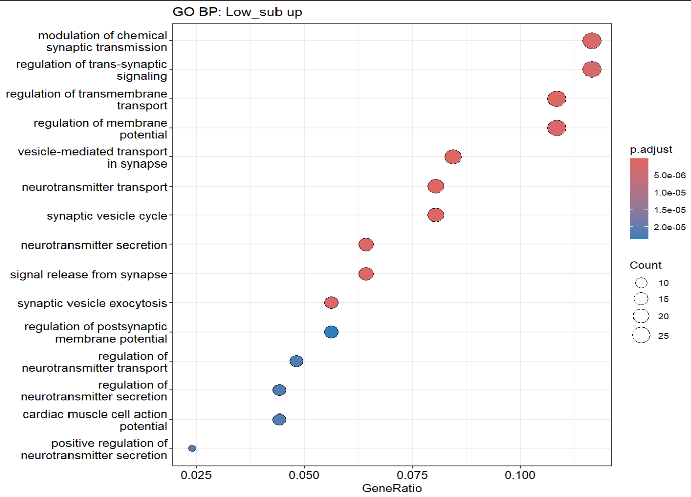
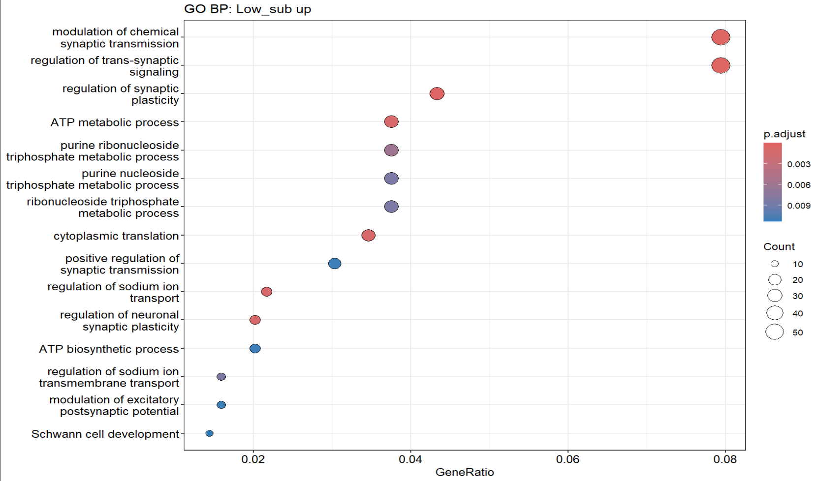
dotplot(ego_low, showCategory = 15) + ggplot2::ggtitle("GO BP: Low_sub up")
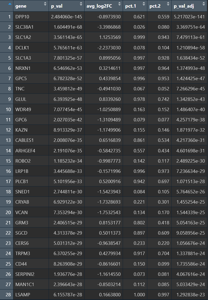
- high_sub更像“稳态/成熟/神经递质代谢型Astro”
- SLC1A2、SLC1A3:谷氨酸转运(稳态Astro核心功能)
- GLUL:谷氨酰胺合成(谷氨酸-谷氨酰胺循环)
- GRM3、PLCB1:代谢/信号传导相关的astro稳态程序
- TRPM3 等:也更偏“成熟astro功能性表达”
- low_sub 更像“反应性/ECM重塑/应激型Astro”
- VCAN、TNC、CD44、SNED1:ECM/细胞外基质与组织重塑、黏附
- CRYAB:应激/伴侣蛋白,反应性astro常见
- SERPINI2、MAN1C1、CERS6等:也更偏应激/代谢重编程背景
- 但是GO富集分析的结果中还是有大量的“神经元突触模块”
- High_sub up组除了和Low_sub有重叠的“突触/神经元模块”,还有“血管/BBB运输+脂代谢(胆固醇合成)”,在之前的教程复现中,确实是有类似的结果,但也需注意是不是混入了其它类型的细胞
meta <- scRNA_astro_clean@meta.data
meta$herv_expr_resid <- resid(lm(herv_expr_score ~ log1p(nCount_RNA) + percent_mito, data=meta))
scRNA_astro_clean$herv_expr_resid <- meta$herv_expr_resid
score_col <- "herv_expr_resid"
# 为了方便计算,这里只取上面deg的显著基因
cand_genes <- deg$gene
# 细胞级
mat <- GetAssayData(scRNA_astro_clean, slot="data")[cand_genes, , drop=FALSE]
meta <- scRNA_astro_clean@meta.data
meta$group <- factor(meta$group)
fit_one_gene <- function(g){
  y <- as.numeric(mat[g, ])
  df <- data.frame(y=y,
                   herv=meta[[score_col]],
                   group=meta$group,
                   nCount=log1p(meta$nCount_RNA),
                   mt=meta$percent_mito)
  m <- lm(y ~ herv + group + nCount + mt, data=df)
  s <- summary(m)$coefficients
  c(beta_herv=s["herv","Estimate"], p_herv=s["herv","Pr(>|t|)"])
}
res_cell <- t(sapply(cand_genes, fit_one_gene)) |> as.data.frame()
res_cell$gene <- rownames(res_cell)
res_cell$padj <- p.adjust(res_cell$p_herv, "BH")
res_cell <- res_cell %>%
  arrange(padj) %>%
  filter(!grepl("^(ENSG|MT-|LINC)|^(AC|AL)[0-9]", gene))
# 样本级
meta <- scRNA_astro_clean@meta.data
pb_score <- meta %>%
  group_by(orig.ident, group) %>%
  summarise(herv = mean(.data[[score_col]]),
            n_cells = n(),
            .groups="drop")
avg_rna <- AverageExpression(scRNA_astro_clean, assays="RNA", slot="data", group.by="orig.ident")[["RNA"]]
samples <- intersect(colnames(avg_rna), pb_score$orig.ident)
pb_score <- pb_score %>% filter(orig.ident %in% samples) %>% arrange(match(orig.ident, samples))
avg_rna  <- avg_rna[cand_genes, samples, drop=FALSE]
fit_one <- function(y, herv, group) {
  df <- data.frame(y=y, herv=herv, group=group)
  m <- lm(y ~ herv + group, data=df)
  s <- summary(m)$coefficients
  c(beta_herv = s["herv","Estimate"], p_herv = s["herv","Pr(>|t|)"])
}
res <- t(sapply(rownames(avg_rna), function(g){
  fit_one(avg_rna[g, ], herv = pb_score$herv, group = pb_score$group)
})) |> as.data.frame()
res$gene <- rownames(res)
res$padj <- p.adjust(res$p_herv, "BH")
res <- res %>%
  arrange(padj) %>%
  filter(!grepl("^(ENSG|MT-|LINC)|^(AC|AL)[0-9]", gene))
# 保存结果
save(res_cell, res, file = "C:\\Users\\17185\\Desktop\\hERV_calc\\GSE157827\\my_data\\0123_3.RData")
- 样本级结果不显著,beta较大,感觉是表达量(hERV分数)加和之后因为某些原因导致和基因计数的量纲不同,之后就不用这种方法了
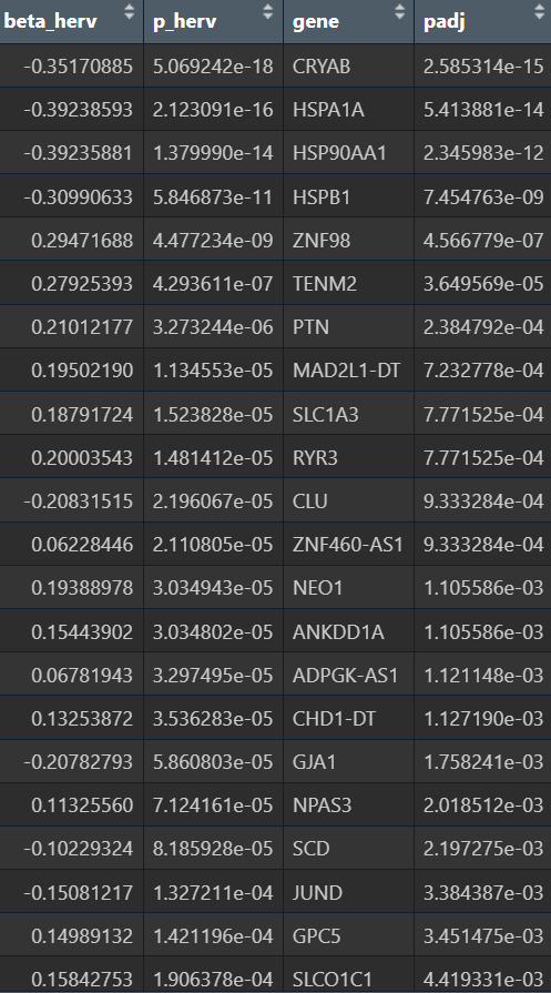
- 细胞级的结果比较正常
- 强负相关(hERV↑,基因↓):CRYAB、HSPA1A/HSP90AA1/HSPB1(热休克蛋白/伴侣蛋白)、CLU、JUND等,这类基因组合很像“应激/蛋白折叠压力/反应性模块”
- 正相关(hERV↑,基因↑):SLC1A3/GJA1(偏Astro/胶质相关)、PTN/NEO1/RYR3/TENM2/NPAS3(偏神经发育/神经相关调控)
与之前GO的结果相似
接下来做几个验证
HERV-high/low的差异是不是“神经元/血管/少突污染”导致
# 点图看表达量
markers_check <- c(
# Astro
"AQP4","GFAP","SLC1A2","SLC1A3","ALDH1L1","CLU",
# Neuron (excit/inhib)
"RBFOX3","SNAP25","SYT1","SLC17A7","GAD1","GAD2",
# Endo / vascular
"PECAM1","VWF","KDR",
# Oligo
"MBP","PLP1","MOG"
)
scRNA_astro_clean$HERV_state_sub <- replace_na(scRNA_astro_clean$HERV_state_sub,"NA")
DotPlot(scRNA_astro_clean, features = markers_check, group.by = "HERV_state_sub") + RotatedAxis()
# 计算模块分数,看high/low是否差别大
gene_sets <- list(
Neuron = intersect(c("RBFOX3","SNAP25","SYT1","SLC17A7","GAD1","GAD2"), rownames(scRNA_astro_clean)),
Endo = intersect(c("PECAM1","VWF","KDR"), rownames(scRNA_astro_clean)),
Oligo = intersect(c("MBP","PLP1","MOG"), rownames(scRNA_astro_clean)),
Astro = intersect(c("AQP4","GFAP","SLC1A2","SLC1A3","ALDH1L1"), rownames(scRNA_astro_clean))
)
DefaultAssay(scRNA_astro_clean) <- "RNA"
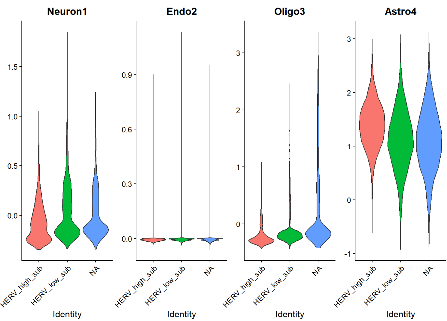
scRNA_astro_clean <- AddModuleScore(scRNA_astro_clean, features = gene_sets, name = names(gene_sets))
VlnPlot(scRNA_astro_clean, features = c("Neuron1", "Endo2", "Oligo3", "Astro4"), group.by = "HERV_state_sub", pt.size = 0, ncol = 4)

共表达是不是被某一两个亚群单独驱动
genes_cand <- c(
  "CRYAB","HSPA1A","HSP90AA1","HSPB1","CLU","JUND","SCD",
  "SLC1A3","GJA1","PTN","NEO1","RYR3","NPAS3","TENM2"
)
genes_cand <- intersect(genes_cand, rownames(scRNA_astro_clean))
expr <- GetAssayData(scRNA_astro_clean, slot="data")[genes_cand, , drop=FALSE]
meta <- scRNA_astro_clean@meta.data %>%
  mutate(
    herv = .data[[score_col]],
    nCount = log1p(nCount_RNA),
    mt = percent_mito,
    group = factor(group),
    sle_reso = as.character(sle_reso)
  )
fit_gene_in_cluster <- function(g, cl){
  idx <- which(meta$sle_reso == cl)
  if(length(idx) < 50) return(NULL)
  y <- as.numeric(expr[g, idx])
  df <- data.frame(y=y, herv=meta$herv[idx], group=meta$group[idx],
                   nCount=meta$nCount[idx], mt=meta$mt[idx])
  m <- lm(y ~ herv + group + nCount + mt, data=df)
  s <- summary(m)$coefficients
  data.frame(
    sle_reso = cl, gene = g,
    beta_herv = s["herv","Estimate"],
    p_herv = s["herv","Pr(>|t|)"],
    n_cells = length(idx)
  )
}
res_by_cluster <- bind_rows(lapply(unique(meta$sle_reso), function(cl){
  bind_rows(lapply(genes_cand, function(g) fit_gene_in_cluster(g, cl)))
}))
res_by_cluster <- res_by_cluster %>%
  group_by(gene) %>%
  mutate(padj_within_gene = p.adjust(p_herv, "BH")) %>%
  ungroup()
View(res_by_cluster %>% arrange(gene, padj_within_gene))
ggplot(res_by_cluster, aes(x=sle_reso, y=beta_herv)) +
  geom_hline(yintercept=0, linetype=2) +
  geom_point(aes(size=-log10(p_herv))) +
  facet_wrap(~gene, scales="free_y") +
  theme_bw() + theme(axis.text.x = element_text(angle=60, hjust=1))
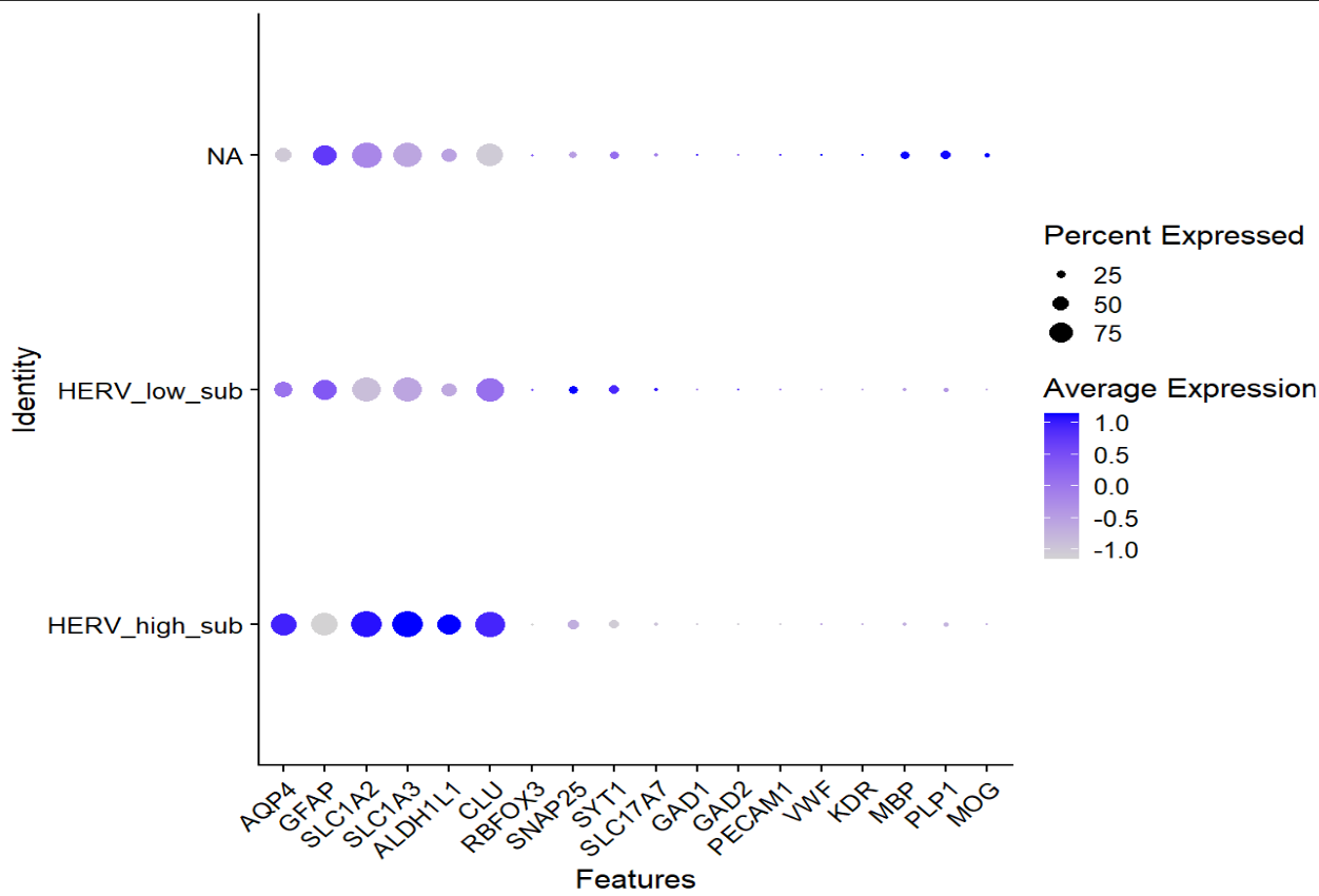

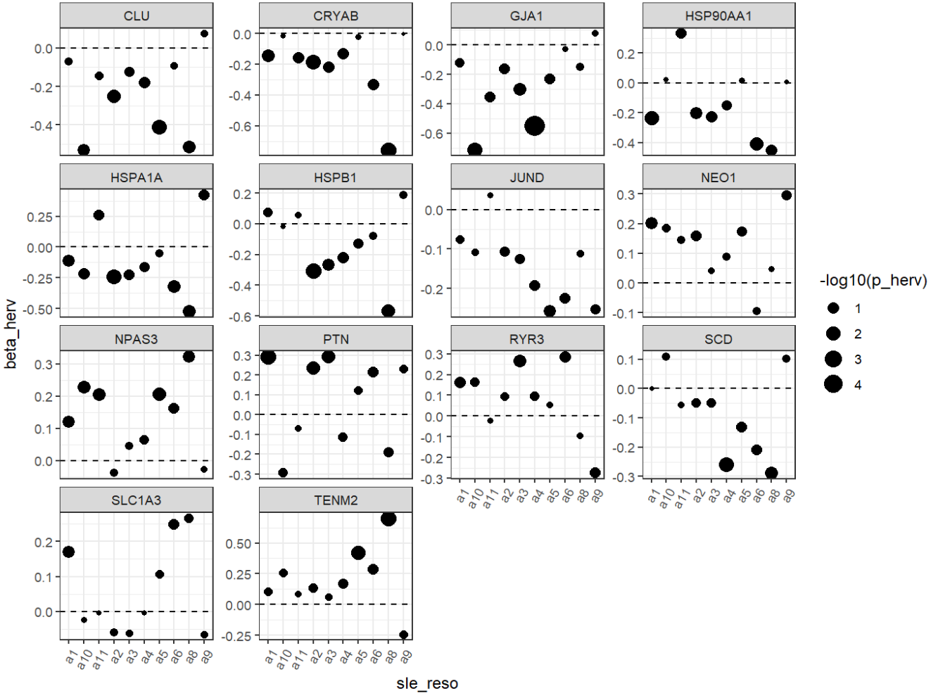
- HERV-high/low并没有哪一个特别偏向“非astro细胞”
- 分布的主要差异确实集中在astro内(看坐标轴刻度),说明这个herv_expr_score的信号主要就是Astro内部变化
- 同一批基因在不同astro子群里,和hERV分数的关联强弱/方向不一样,说明“hERV分数—基因表达”关系是有亚群依赖的
一些问题:
- 上面的共表达分析使用
meta$herv_expr_resid <- resid(lm(herv_expr_score ~ log1p(nCount_RNA) + percent_mito, data=meta))这段代码,目的是把herv里能被库深度/线粒体解释掉的部分剔除,而之后又lm(y ~ herv + group + nCount + mt, data=df)又把这些协变量放回来了,因此之前的残差化是没有必要的 -
在最初计算
herv_expr_score时,是直接用选出的hERV家族的data计数取平均值,而这些hERV家族有一些是AD上调、一些是AD下调,如果想研究带有“AD/NC”信息的hERV分数,就不应混起来算,可以把score_ADup-score_ADdown作为总分然而在后面实测时,发现
score_ADup和score_ADdown是直接取计数平均值算出来的,而down的hERV家族有8个,up的只有2个,平均值相减后导致up的权重上升,最后的结果反而没之前显著了。因此最后决定就用down(AD下调)的几个家族,这样的分数就是越小越偏AD
assay_herv <- "HERV_family"
assay_rna  <- "RNA"
astro_sub_col <- "sle_reso"
DefaultAssay(scRNA_astro_clean) <- assay_herv
# 选出HERV家族
panel <- c("HML1","HML3","HML4","HERVK14C","MER101","HERVH48","MER41","HERVW","HARLEQUIN","HERVEA")
up_set <- c("HARLEQUIN","HERVEA")  # AD中上调
down_set <- c("HML1","HML3","HML4","HERVK14C","MER101","HERVH48","MER41","HERVW")  # AD中下调
# 计算分数
Xd <- GetAssayData(scRNA_astro_clean, assay = assay_herv, slot = "data")[panel, , drop = FALSE]
Xc <- GetAssayData(scRNA_astro_clean, assay = assay_herv, slot = "counts")[panel, , drop = FALSE]
scRNA_astro_clean$herv_expr_score <- Matrix::colMeans(Xd)
scRNA_astro_clean$herv_detect_score <- Matrix::colMeans(Xc > 0)
scRNA_astro_clean$herv_up_expr <- Matrix::colMeans(Xd[up_set, , drop=FALSE])
scRNA_astro_clean$herv_up_detect <- Matrix::colMeans(Xc[up_set, , drop=FALSE] > 0)
scRNA_astro_clean$herv_down_expr <- Matrix::colMeans(Xd[down_set, , drop=FALSE])
scRNA_astro_clean$herv_down_detect <- Matrix::colMeans(Xc[down_set, , drop=FALSE] > 0)
scRNA_astro_clean$herv_expr_score_dir <- scRNA_astro_clean$herv_up_expr - scRNA_astro_clean$herv_down_expr
scRNA_astro_clean$herv_detect_score_dir <- scRNA_astro_clean$herv_up_detect - scRNA_astro_clean$herv_down_detect
# 根据down分数的差值划分类群,分数越小越偏AD
make_state <- function(x, q_lo = 0.2, q_hi = 0.8) {
  lo <- quantile(x, q_lo, na.rm = TRUE)
  hi <- quantile(x, q_hi, na.rm = TRUE)
  ifelse(x >= hi, "high", ifelse(x <= lo, "low", "mid"))
}
metaA <- scRNA_astro_clean@meta.data %>%
  mutate(
    astro_sub = factor(.data[[astro_sub_col]]),
    group = factor(group, levels = c("NC","AD"))
  )
metaA$herv_state <- make_state(metaA$herv_down_expr)
# 各子群AD-NC的差异
tab1 <- prop.table(table(metaA$herv_state, metaA[[astro_sub_col]]), 2)
tab2 <- prop.table(table(metaA$herv_state, metaA$group), 2)
> tab1
              a1       a10       a11        a2        a3
  high 0.1962328 0.3888889 0.3631436 0.1511989 0.1285874
  low  0.4259207 0.1161616 0.1327913 0.5269394 0.5262766
  mid  0.3778465 0.4949495 0.5040650 0.3218618 0.3451360
              a4        a5        a6        a8        a9
  high 0.3260638 0.1961031 0.2384314 0.1468085 0.2281450
  low  0.1946809 0.3821496 0.3129412 0.5319149 0.2046908
  mid  0.4792553 0.4217473 0.4486275 0.3212766 0.5671642
> tab2
              NC        AD
  high 0.2412145 0.1644172
  low  0.3586563 0.4554378
  mid  0.4001292 0.3801450
Astro各子群里AD-NC的分数差异
# 每个子群里的分布
ggplot(metaA, aes(x = group, y = herv_down_expr, fill = group)) +
  geom_violin(scale = "width", trim = TRUE) +
  geom_boxplot(width = 0.18, outlier.size = 0.2) +
  facet_wrap(~ astro_sub, ncol = 4, scales = "free_y") +
  stat_compare_means(method = "t.test", label = "p.signif") +
  theme_classic() +
  xlab(NULL) + ylab("herv_expr_score")
# 每个子群做Wilcoxon
safe_wilcox <- function(df){
  tryCatch(wilcox.test(herv_down_expr ~ group, data = df)$p.value, error = function(e) NA_real_)
}
res_sub_cell_wilcox <- metaA %>%
  group_by(astro_sub) %>%
  summarise(
    n_NC = sum(group=="NC"),
    n_AD = sum(group=="AD"),
    med_NC = median(herv_down_expr[group=="NC"]),
    med_AD = median(herv_down_expr[group=="AD"]),
    delta_median = med_AD - med_NC,
    p = safe_wilcox(cur_data()),
    .groups = "drop"
  ) %>%
  mutate(p_adj = p.adjust(p, method = "BH")) %>%
  arrange(p_adj)
能区分某些亚群里的AD-NC状态?(至少在细胞层面,在样本层面仍不显著)
# hERV-high和low的差异基因:与之前选几个亚群来比不同,这里直接比较herv_state的low和high
DefaultAssay(scRNA_astro_clean) <- "RNA"
scRNA_astro_clean$herv_state <- metaA$herv_state
Idents(scRNA_astro_clean) <- "herv_state"
deg <- FindMarkers(
  scRNA_astro_clean,
  ident.1 = "high",
  ident.2 = "low",
  test.use = "MAST",
  latent.vars = c("orig.ident", "nCount_RNA", "percent_mito"),
  logfc.threshold = 0.1,
  min.pct = 0.05
)
deg <- deg %>%
  tibble::rownames_to_column("gene") %>%
  arrange(p_val_adj) %>%
  filter(!grepl("^(ENSG|MT-|LINC)|^(AC|AL)[0-9]", gene))
save(deg, file = "C:\\Users\\17185\\Desktop\\hERV_calc\\GSE157827\\my_data\\0125_2.RData")
# GO分析
deg_sig <- deg %>%
  filter(p_val_adj<0.05, abs(avg_log2FC)>0.25)
genes_high_up <- deg_sig %>% filter(avg_log2FC > 0) %>% pull(gene) %>% unique()  # hERV分数更高(偏向NC)的细胞上调的基因
genes_low_up  <- deg_sig %>% filter(avg_log2FC < 0) %>% pull(gene) %>% unique()  # hERV分数更低(偏向AD)的细胞上调的基因
DefaultAssay(scRNA_astro_clean) <- "RNA"
expr_counts <- GetAssayData(scRNA_astro_clean, slot = "counts")
universe <- rownames(expr_counts)[Matrix::rowSums(expr_counts > 0) >= 10]
ego_high <- enrichGO(
  gene      = genes_high_up,
  universe  = universe,
  OrgDb     = org.Hs.eg.db,
  keyType   = "SYMBOL",
  ont       = "BP",
  pAdjustMethod = "BH",
  pvalueCutoff   = 1,
  qvalueCutoff   = 1,
  readable = TRUE
)
ego_low <- enrichGO(
  gene      = genes_low_up,
  universe  = universe,
  OrgDb     = org.Hs.eg.db,
  keyType   = "SYMBOL",
  ont       = "BP",
  pAdjustMethod = "BH",
  pvalueCutoff   = 1,
  qvalueCutoff   = 1,
  readable = TRUE
)
dotplot(ego_high, showCategory = 15) + ggplot2::ggtitle("GO BP: High_sub up")
dotplot(ego_low,  showCategory = 15) + ggplot2::ggtitle("GO BP: Low_sub up")
# 共表达
meta <- scRNA_astro_clean@meta.data
meta$group <- factor(meta$group)
score_col <- "herv_down_expr"
# 取目标基因
load("C:\\Users\\17185\\Desktop\\hERV_calc\\GSE157827\\my_data\\0125_2.RData")
deg <- deg %>%
  filter(p_val_adj<0.05)
cand_genes <- deg$gene
# 细胞级
DefaultAssay(scRNA_astro_clean) <- "RNA"
mat <- GetAssayData(scRNA_astro_clean, slot="data")[cand_genes, , drop=FALSE]
fit_one_gene <- function(g){
  y <- as.numeric(mat[g, ])
  df <- data.frame(y=y,
                   herv=meta[[score_col]],
                   group=meta$orig.ident,  # 和前面FindMarkers统一,都使用这三个协变量
                   nCount=log1p(meta$nCount_RNA),
                   mt=meta$percent_mito)
  m <- lm(y ~ herv + group + nCount + mt, data=df)
  s <- summary(m)$coefficients
  c(beta_herv=s["herv","Estimate"], p_herv=s["herv","Pr(>|t|)"])
}
res_cell <- t(sapply(cand_genes, fit_one_gene)) |> as.data.frame()
res_cell$gene <- rownames(res_cell)
res_cell$padj <- p.adjust(res_cell$p_herv, "BH")
res_cell <- res_cell %>%
  arrange(padj) %>%
  filter(!grepl("^(ENSG|MT-|LINC)|^(AC|AL)[0-9]", gene))
# 保存结果
save(res_cell, file = "C:\\Users\\17185\\Desktop\\hERV_calc\\GSE157827\\my_data\\0125_1.RData")
write.csv(res_cell %>% filter(padj<0.05), file.path(res_dir, "res_cell_0125.csv"), row.names = F)
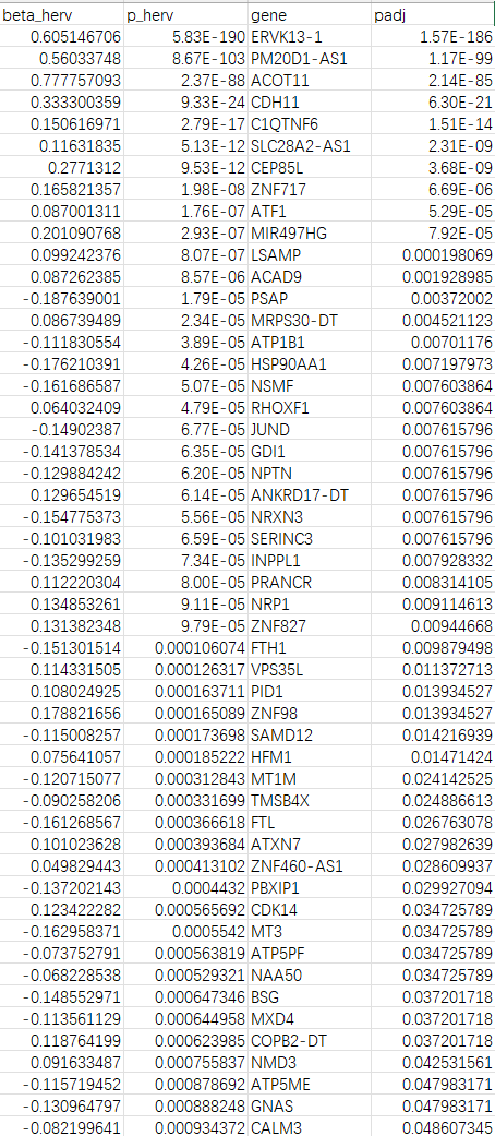
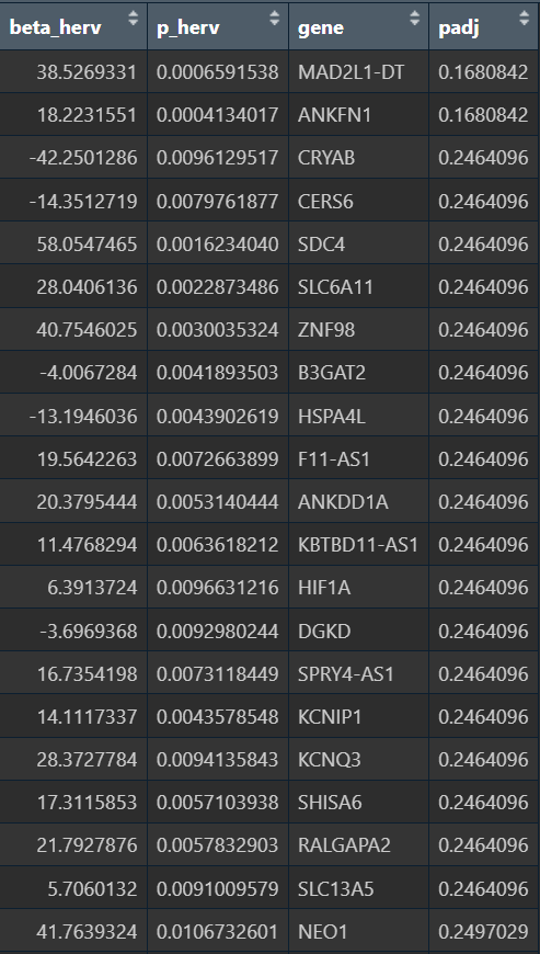
-
hERV得分low的细胞(更偏向AD的细胞)相对上调的基因显著富集于“突触相关信号调控/离子转运/能量代谢与翻译”等过程,提示HERV-low更偏向某种“神经活动/代谢-翻译活跃”的细胞状态
不过可能与细胞状态/混杂有关,后续可用neuron marker排查
- hERV得分high的细胞呈现脂质分解/脂肪酸氧化/血管相关迁移等趋势,但富集结果不显著,可能因为上调基因数量较少/功能异质/阈值切分导致信号分散
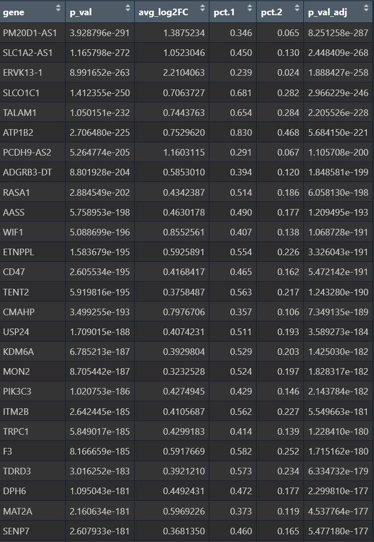
- 正相关(hERV分数↑,基因↑):
- ERVK13-1:可能也属于ERV/TE序列,所以相关度较高
- ACOT11/ACAD9:脂质/脂肪酸氧化
- CDH11:细胞黏附/状态改变
- PM20D1-AS1:神经退行/代谢相关
- 负相关(hERV分数↑,基因↓):
- ATP5PF/ATP5ME(线粒体ATP合成相关):与前面GO富集“ATP metabolic/biosynthetic process” 的方向是一致的。HERV分数越高,ATP合成/能量相关基因越低?
- FTL/FTH1(铁蛋白)、MT3/MT1M(金属硫蛋白)、HSP90AA1(伴侣蛋白)、PSAP(溶酶体/脂代谢相关):属于“应激/金属-氧化还原/蛋白稳态/溶酶体相关”的大类
- APOE:在第一次没把样本加入协变量时(
y ~ herv + group + nCount + mt),padj<0.05,之后padj≈0.1。在共表达结果中,hERV分数越高(越偏向正常),它表达越低,但在上面的deg结果中,它的logFC却>0,说明在hERV分数高的细胞中表达量高
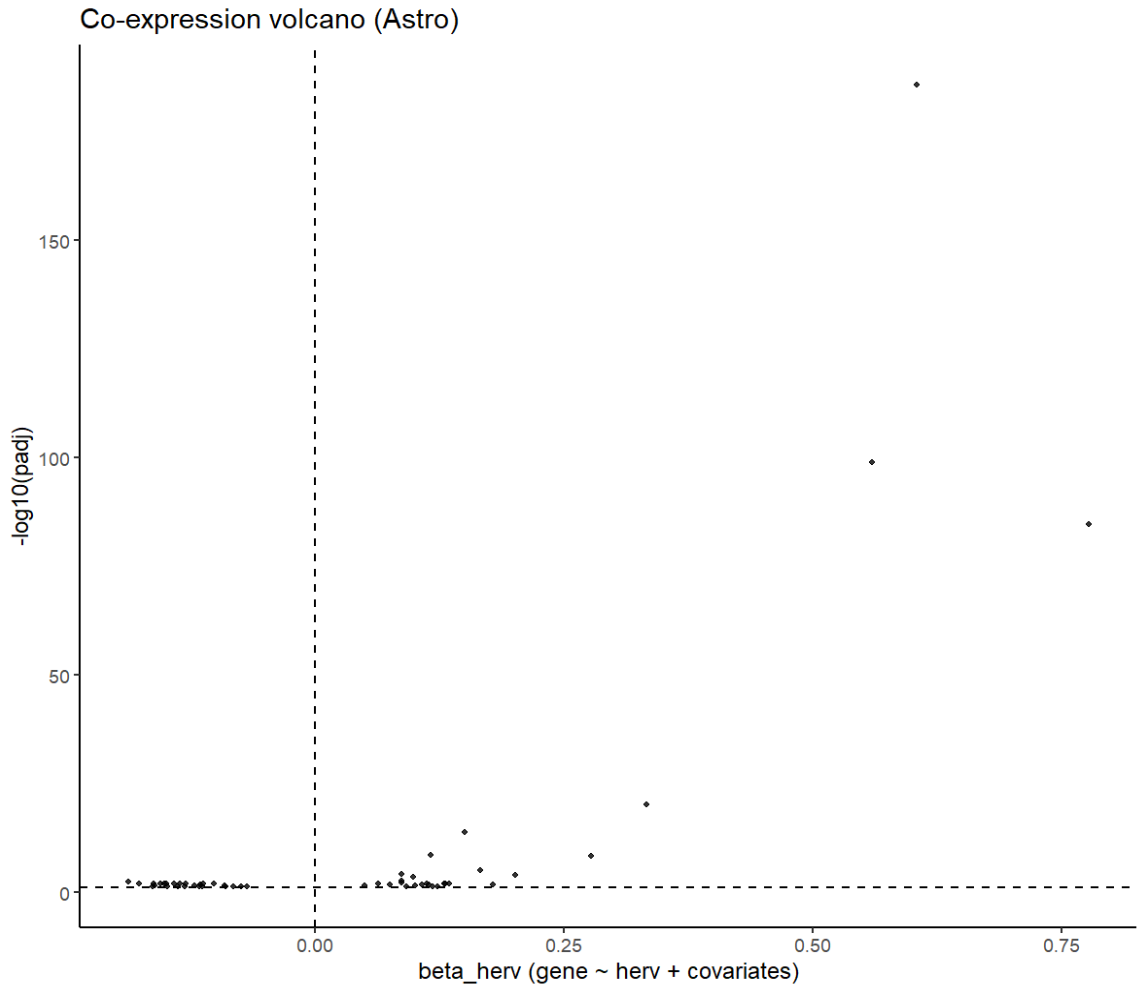
简单画几张结果展示图
res_cell <- read.csv(file.path(res_dir, "res_cell_0125.csv"), stringsAsFactors = FALSE)
label_genes <- c("ACOT11","CDH11","FTL","FTH1","MT3","APOE","ATP5PF","ATP5ME","ACAD9")
# 火山图
res_cell %>%
  mutate(
    neglog10_padj = -log10(padj),
    sig = padj < 0.05
  ) %>%
  ggplot(aes(x = beta_herv, y = neglog10_padj)) +
  geom_point(aes(alpha = sig), size = 1) +
  scale_alpha_manual(values = c(`TRUE` = 0.8, `FALSE` = 0.25), guide = "none") +
  geom_vline(xintercept = 0, linetype = 2) +
  geom_hline(yintercept = -log10(0.05), linetype = 2) +
  ggrepel::geom_text_repel(
    data = . %>% filter(gene %in% label_genes),
    aes(label = gene),
    size = 3,
    max.overlaps = Inf
  ) +
  labs(
    x = "beta_herv (gene ~ herv + covariates)",
    y = "-log10(padj)",
    title = "Co-expression volcano (Astro)"
  ) +
  theme_classic()
# 取几个基因画全体细胞散点图+线性拟合(按group上色)
plot_gene_vs_herv <- function(gene){
  stopifnot(gene %in% rownames(mat))
  df <- data.frame(
    cell = colnames(mat),
    expr = as.numeric(mat[gene, colnames(mat)]),
    herv = meta[colnames(mat), score_col],
    group = meta[colnames(mat), "group"],
    sle_reso = meta[colnames(mat), "sle_reso"],
    nCount_RNA = meta[colnames(mat), "nCount_RNA"],
    percent_mito = meta[colnames(mat), "percent_mito"]
  )
  p <- ggplot(df, aes(x = herv, y = expr, color = group)) +
    geom_point(size = 0.4, alpha = 0.25) +
    geom_smooth(method = "lm", se = FALSE) +
    labs(
      title = paste0(gene, " vs ", score_col),
      x = score_col,
      y = paste0(gene, " expression (Seurat data slot)")
    ) +
    theme_classic() +
    facet_wrap(~ sle_reso, scales = "free_y")
}
print(plot_gene_vs_herv("ACOT11"))
print(plot_gene_vs_herv("CDH11"))
print(plot_gene_vs_herv("FTL"))
print(plot_gene_vs_herv("MT3"))
print(plot_gene_vs_herv("APOE"))
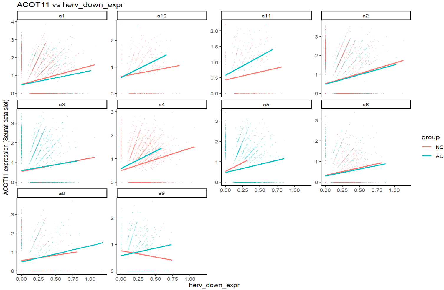
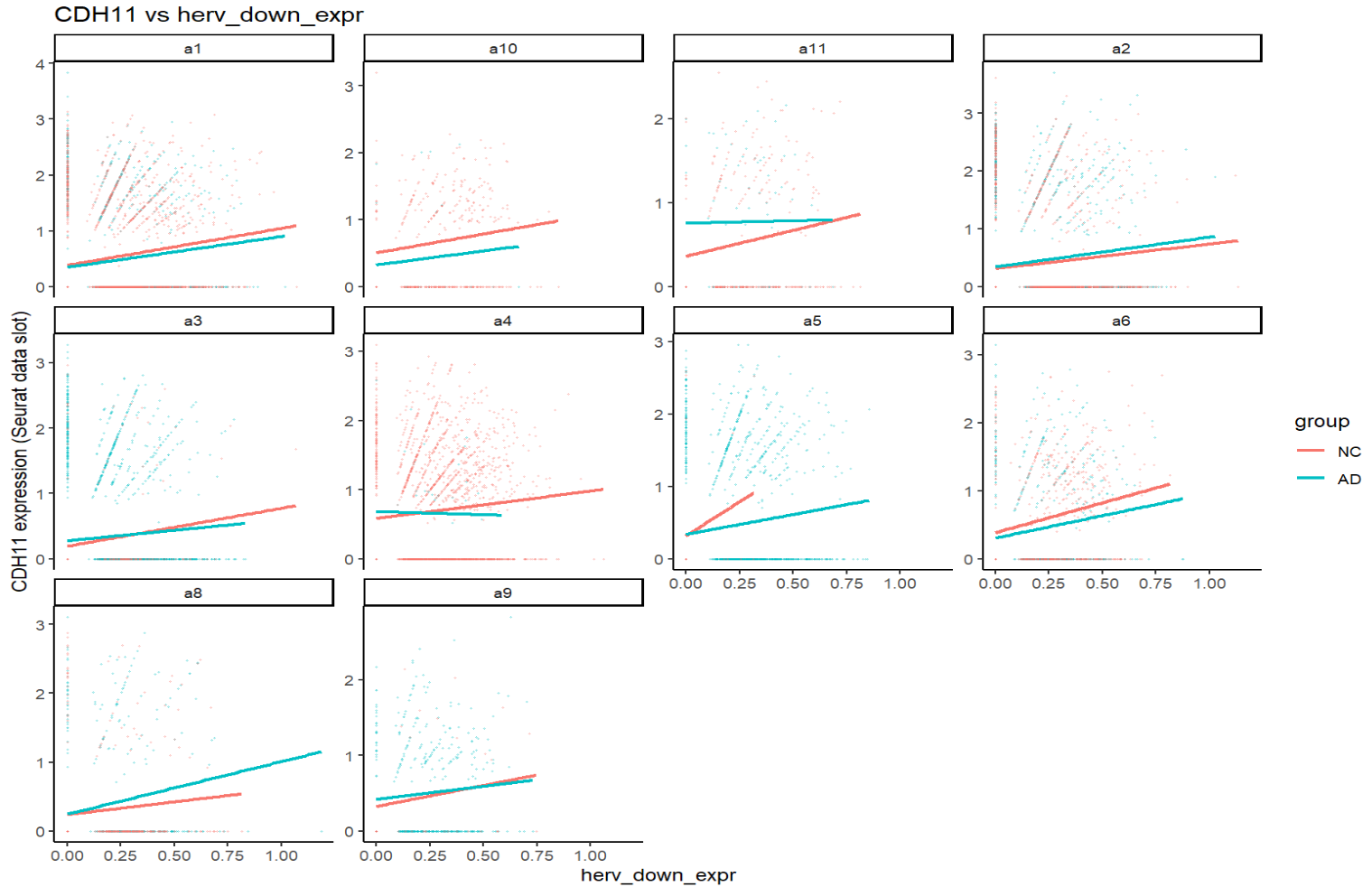
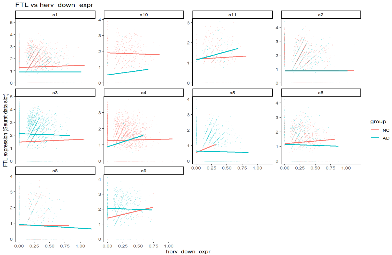
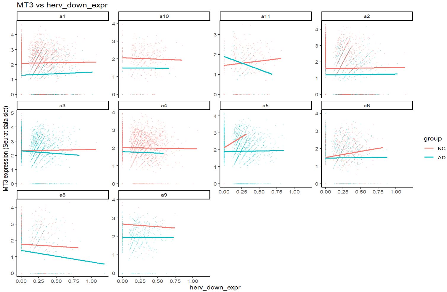
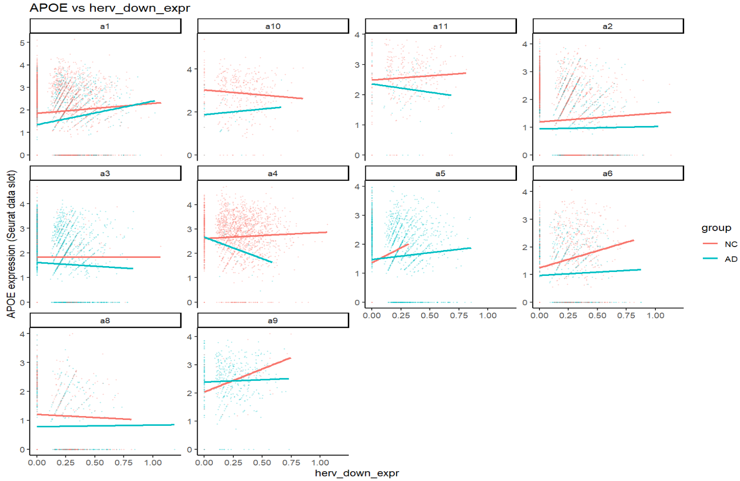
关键:一个基因在不同亚群、不同分组(NC/AD)下,斜率常常不同,方向有时也不同。这就可能导致APOE这样在两个结果中方向相反的问题(FindMarkers是high组平均表达-low组平均表达,而high/low两组在同一亚群中构成比例不同)
- 后面做这类分析,可以把group/sle_reso也列入协变量
一些补充讨论:
- 根据low-high画一个astro内的umap图
- 之前我们做了“Astro各子群里AD-NC的分数差异”,现在我想对所有细胞按这个方法计算分数,看在其它的亚群中,这个分数能否区分AD-NC
# high-low-mid三种状态的分布
Idents(scRNA_astro_clean) <- "herv_state"
DimPlot(scRNA_astro_clean, reduction = "umap", group.by = "herv_state") / DimPlot(scRNA_astro_clean, reduction = "umap", group.by = "herv_state", split.by = "group")
# 取出high和low细胞
scRNA_astro_clean2 <- subset(scRNA_astro_clean, subset = herv_state %in% c("high","low"))
Idents(scRNA_astro_clean2) <- "herv_state"
# 看high-low的划分与AD-NC划分的区别
DimPlot(scRNA_astro_clean2, reduction = "umap", group.by = "herv_state", split.by = "herv_state") / DimPlot(scRNA_astro_clean2, reduction = "umap", group.by = "herv_state", split.by = "group") /  DimPlot(scRNA_astro_clean2, reduction = "umap", group.by = "group", split.by = "group")
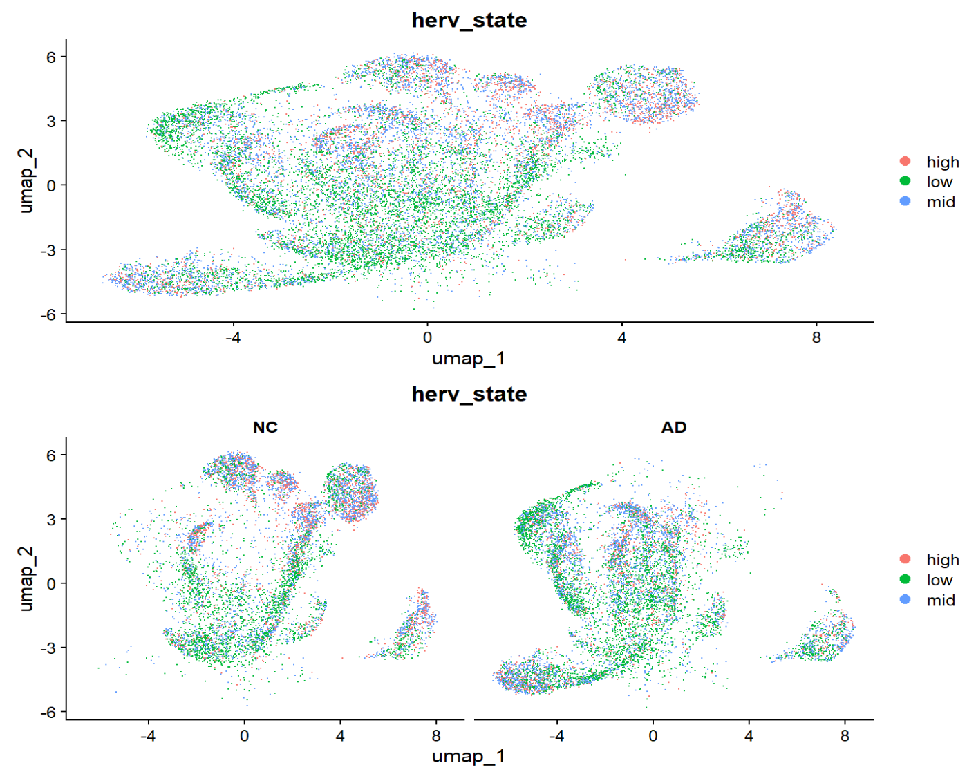
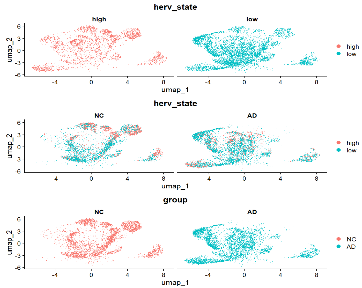
high-low的分布与NC-AD的分布还是挺对应的
# 计算分数
DefaultAssay(seu) <- "HERV_family"
herv_mat <- GetAssayData(seu, slot = "data")
seu$herv_down_expr <- Matrix::colMeans(herv_mat[down_set, , drop = FALSE])
seu$herv_state <- make_state(seu$herv_down_expr)
meta_all <- seu@meta.data %>%
  mutate(
    group = factor(group, levels = c("NC","AD")),
    celltype = factor(celltype)
  )
# 每个细胞类型内AD-NC的herv_down_expr
ggplot(meta_all, aes(x = celltype, y = herv_down_expr, fill = group)) +
  geom_violin(scale = "width", trim = TRUE) +
  geom_boxplot(width = 0.15, outlier.size = 0.2, alpha = 0.4) +
  stat_compare_means(method = "t.test", label = "p.signif") +
  theme_bw() +
  theme(axis.text.x = element_text(angle = 45, hjust = 1)) +
  labs(title = "HERV down score across cell types (AD vs NC)",
       y = "herv_down_expr")
# 看一下具体的p值
stat_celltype <- meta_all %>%
  group_by(celltype) %>%
  summarise(
    n_NC = sum(group=="NC"),
    n_AD = sum(group=="AD"),
    p_wilcox = tryCatch(wilcox.test(herv_down_expr ~ group)$p.value, error=function(e) NA_real_),
    effect_median = mean(herv_down_expr[group=="AD"], na.rm=TRUE) -
                    mean(herv_down_expr[group=="NC"], na.rm=TRUE),
    .groups = "drop"
  ) %>%
  mutate(padj = p.adjust(p_wilcox, method = "BH")) %>%
  arrange(padj)
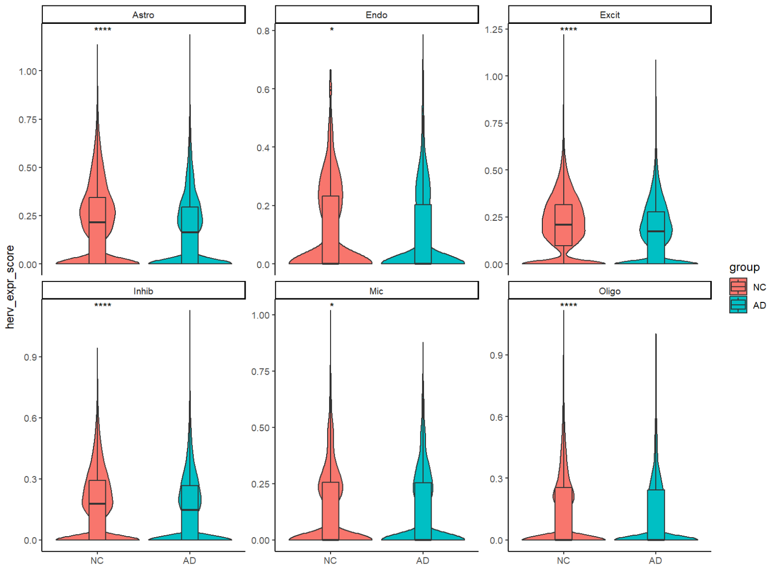
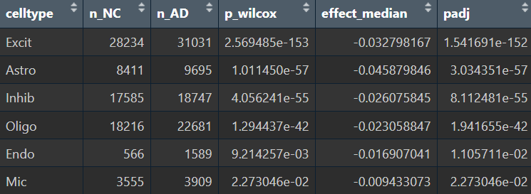
在细胞数较多的主要细胞类型中,这个分数还是能比较显著地区分AD-NC的,且AD的均分都要等于NC,和假设相符
other try
有没有哪些细胞类型/亚群”的hERV得分有差别
主要问题:这个hERV分数是直接拿count算的,所以会受总体测序深度的影响,在比较hERV分数时可能要考虑这个影响差点被GPT误导了,这个分数虽然确实是直接对计数取平均值,不过我们的计数(data层)已经是用RNA的库深度(nCount_RNA)做了LogNormalize的,所以这个影响感觉并没有那么大,不过根据GPT的说法,nCount_RNA仍然常常和很多“细胞状态/检测率/零膨胀”相关,可能有残留,所以在分析时还是要考虑一下测序深度的影响(就像之前找high-low的差异基因和共表达那样)
探讨某个亚群/细胞大类的hERV得分的不同时,应该是把这个亚群/细胞大类和其它的亚群/细胞大类,而不是两两比较?
score_col <- "herv_down_expr"
subcol <- "sle_reso"
group_col <- "group"
ncount_col <- "nCount_RNA"
mt_col <- "percent_mito"
sample_col <- "orig.ident"
celltype_col<- "celltype"
one_vs_rest_lm <- function(df, score="herv_down_expr", class="sub", covars=c("group","log_nCount","mt","sample")) {
# one_vs_rest_lm <- function(df, score="herv_down_expr", class="sub", covars=c("log_nCount","mt","sample")) {
y <- df[[score]]
levs <- levels(df[[class]])
res <- lapply(levs, function(k){
is_k <- as.integer(df[[class]] == k)
dat <- df %>% mutate(is_k = is_k)
fml <- as.formula(
paste0("y ~ is_k + ", paste(covars, collapse = " + "))
)
fit <- lm(fml, data = dat)
sm <- summary(fit)$coefficients
data.frame(
class = k,
n_in = sum(is_k==1),
n_out = sum(is_k==0),
beta = sm["is_k","Estimate"],
se = sm["is_k","Std. Error"],
t = sm["is_k","t value"],
p = sm["is_k","Pr(>|t|)"],
stringsAsFactors = FALSE
)
}) %>% bind_rows()
res$padj <- p.adjust(res$p, method = "BH")
res %>% arrange(padj)
}
# astro亚群
metaA <- scRNA_astro_clean@meta.data %>%
mutate(
group = factor(.data[[group_col]], levels = c("NC","AD")),
sub = factor(.data[[subcol]]),
log_nCount = log1p(.data[[ncount_col]]),
mt = .data[[mt_col]],
sample = factor(.data[[sample_col]])
)
res_sub <- one_vs_rest_lm(metaA, score = score_col, class = "sub")
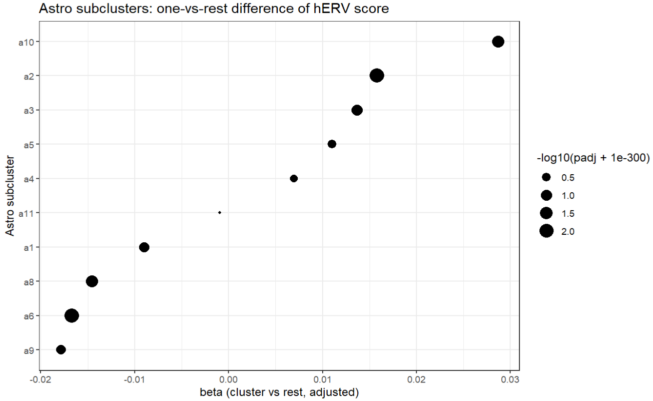
ggplot(res_sub, aes(x = reorder(class, beta), y = beta)) +
geom_point(aes(size = -log10(padj + 1e-300))) +
coord_flip() +
theme_bw() +
labs(x = "Astro subcluster", y = "beta (cluster vs rest, adjusted)",
title = "Astro subclusters: one-vs-rest difference of hERV score")
# 细胞大类
metaAll <- seu@meta.data %>%
  mutate(
    group = factor(.data[[group_col]], levels = c("NC","AD")),
    celltype = factor(.data[[celltype_col]]),
    log_nCount = log1p(.data[[ncount_col]]),
    mt = .data[[mt_col]],
    sample = factor(.data[[sample_col]])
  )
res_celltype <- one_vs_rest_lm(metaAll, score = score_col, class = "celltype")
ggplot(res_celltype, aes(x = reorder(class, beta), y = beta)) +
  geom_point(aes(size = -log10(padj + 1e-300))) +
  coord_flip() +
  theme_bw() +
  labs(x = "Cell type", y = "beta (type vs rest, adjusted)",
       title = "Cell types: one-vs-rest difference of hERV score")
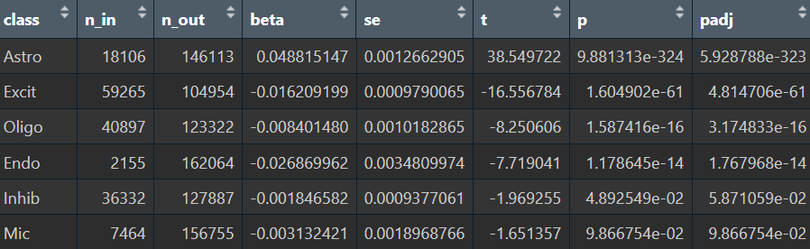
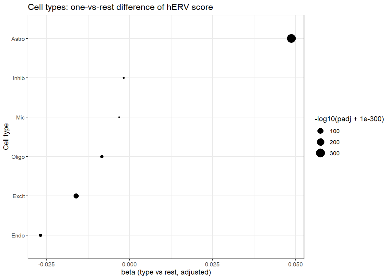
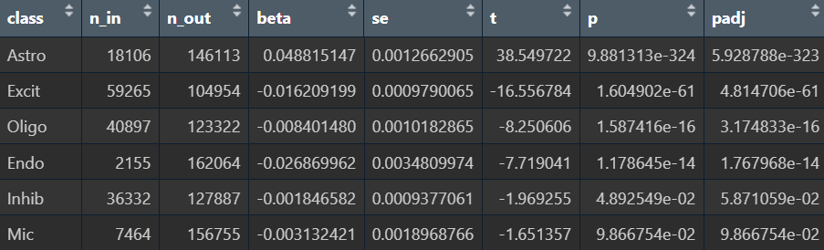
看起来astro确实是hERV表达最不同的那个,从astro开始进行分析确实是对的。除此之外,Endo、Excit和Oligo的差异值和p值都较大
-
不过也需考虑是不是AD-NC的组成差异:这就是为什么要把group加入协变量
          NC    AD
Astro  8411  9695
Endo    566  1589
Excit 28234 31031
Inhib 17585 18747
Mic    3555  3909
Oligo 18216 22681
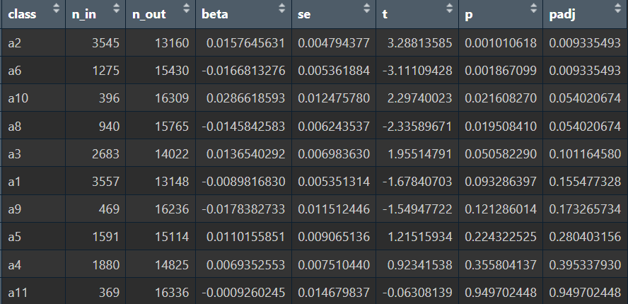
在astro亚群中,a2显著偏高、a6显著偏低,不过比较奇怪的是,这两个亚群的AD-NC数量倒是很平均,应该是因为分析时把group(AD/NC状态)加入了协变量,所以AD-NC数量差异大的都被消除掉了
去掉之后再试一次:
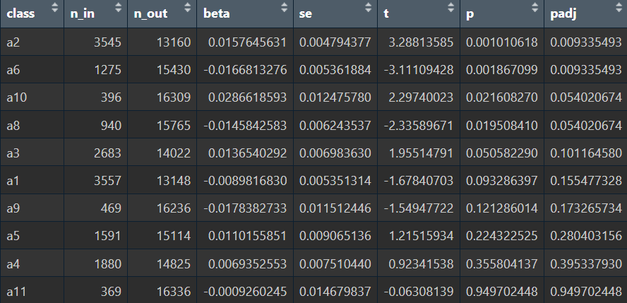
结果并没有太大变化,说明这两个亚群的hERV差异是比较稳定的
再看一下astro各亚群的平均hERV分数
sub_rank <- scRNA_astro_clean@meta.data %>%
  group_by(sle_reso) %>%
  summarise(mean_expr = mean(herv_down_expr),
            n_cells = n(),
            .groups = "drop") %>%
  arrange(desc(mean_expr))
ggplot(sub_rank, aes(x=reorder(sle_reso, mean_expr), y=mean_expr)) +
  geom_col() + coord_flip() + theme_classic() +
  labs(x="Astro subcluster", y="Panel mean expression")
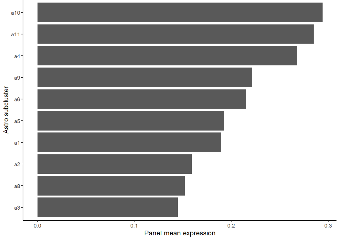
看来这个朴实的平均分数计算的结果和上面用较复杂的方法的结果不太一样,从某种程度上说明加上协变量的影响还是很大的(即使不把group作为协变量),而且上面的方法是一对多的比较(one-vs-rest)
关于上次的一些问题
重合的基因过少,差在哪里
- 去掉版本号
.1 - 差异是否属于以
ENSG开头的无symbol的基因 - 差异是否属于
MT-/RP[SL]开头的线粒体/核糖体基因 - 差异是否属于以
(AC|AL)[0-9]或LINC开头的奇奇怪怪的基因- LINC01053等:长链非编码RNA
- AC136489/AL158055这种:常见的“克隆/基因座式”临时命名(很多是lncRNA、反义转录本、未充分注释的转录本等)
- 除此之外,我还看到差异基因名里有很多以
-DT/-AS1/-AS2结尾的- DT:发散转录本,通常与某个蛋白编码基因共享或靠近同一启动子区域,但在相反方向启动转录。例如AP1AR-DT往往是从AP1AR附近启动子区域向相反方向转录的lncRNA
- AS:某个“主基因”的反义链转录本/基因。例如AP4B1-AS1通常表示位于AP4B1相关区域、并且在基因组上与AP4B1反向链重叠或相邻的lncRNA
总的来说,就是和某个“主基因”在基因组位置/方向上有强关系的一类非编码转录本(很多是lncRNA)
最开始的结果:
ours genes: 21002
auth genes: 17276
common genes: 13938
overlap % (of ours): 66.37 %
overlap % (of auth): 80.68 %
ours_genes <- rownames(mat_ours)
auth_genes <- rownames(mat_auth)
norm_gene <- function(x) {
  str_replace(x, "\\.\\d+$", "")
}
ours_norm <- norm_gene(ours_genes)
auth_norm <- norm_gene(auth_genes)
cat("norm overlap:", length(intersect(ours_norm, auth_norm)), "\n")
# 基因名里有多少是“重复SYMBOL被唯一化”造成的
dup_core <- sum(duplicated(ours_norm))
cat("ours duplicated after norm:", dup_core, " / ", length(ours_norm), "\n")
norm overlap: 13939
ours duplicated after norm: 6  /  21002
影响很小,不是这里的问题
ours_only <- setdiff(ours_norm, auth_norm)
auth_only <- setdiff(auth_norm, ours_norm)
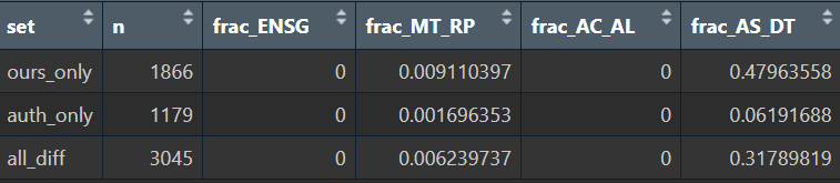
all_diff <- union(ours_only, auth_only)
report_patterns <- function(vec, label) {
tibble(
set = label,
n = length(vec),
frac_ENSG = mean(str_detect(vec, "^ENSG\\d+")),
frac_MT_RP = mean(str_detect(vec, "^(MT-)|^RP[SL]")),
frac_AC_AL = mean(str_detect(vec, "^(AC|AL)[0-9]\\d|^LINC")),
frac_AS_DT = mean(str_detect(vec, "(-AS\\d+)$|(-DT)$"))
)
}
View(bind_rows(
report_patterns(ours_only, "ours_only"),
report_patterns(auth_only, "auth_only"),
report_patterns(all_diff, "all_diff")
))
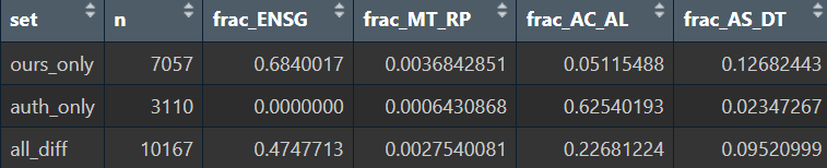
大概6-7成的基因属于ENSG和AC/AL类
ours_filter <- ours_genes[!grepl("^(ENSG|MT-|LINC)|^(AC|AL)[0-9]", ours_genes)]
auth_filter <- auth_genes[!grepl("^(ENSG|MT-|LINC)|^(AC|AL)[0-9]", auth_genes)]
common_genes <- intersect(ours_filter, auth_filter)
cat("common genes:", length(common_genes), "\n")
cat("overlap % (of ours):", round(length(common_genes)/length(ours_filter)*100, 2), "%\n")
cat("overlap % (of auth):", round(length(common_genes)/length(auth_filter)*100, 2), "%\n")
common genes: 13604
overlap % (of ours): 87.94 %
overlap % (of auth): 92.02 %
按我前面常用的基因规则过滤后,相似度显著上升
其实我之前过滤基因名时都用的是AC|AL|LINC|AP,但实际上以AP+数字开头的都不是非编码基因,比如AP4B1这种,不过这些基因一共也就30个左右,不是很影响总的结果
# 看看剩下的基因都属于哪种情况
ours_filter_only <- setdiff(ours_filter, auth_filter)
auth_filter_only <- setdiff(auth_filter, ours_filter)
all_filter_diff <- union(ours_filter_only, auth_filter_only)
View(bind_rows(
  report_patterns(ours_filter_only, "ours_only"),
  report_patterns(auth_filter_only, "auth_only"),
  report_patterns(all_filter_diff, "all_diff")
))
# 再过滤掉所有的AS/DT
ours_filter_ACAL <- ours_filter[!grepl("(-AS\\d+)$|(-DT)$", ours_filter)]
auth_filter_ACAL <- auth_filter[!grepl("(-AS\\d+)$|(-DT)$", auth_filter)]
common_genes <- intersect(ours_filter_ACAL, auth_filter_ACAL)
cat("common genes:", length(common_genes), "\n")
cat("overlap % (of ours):", round(length(common_genes)/length(ours_filter_ACAL)*100, 2), "%\n")
cat("overlap % (of auth):", round(length(common_genes)/length(auth_filter_ACAL)*100, 2), "%\n")
common genes: 13187
overlap % (of ours): 93.14 %
overlap % (of auth): 92.26 %
剩下的基因就都是比较正常的格式了,这个水平我觉得是可以接受的
多重比对的处理方法
- stellarscope用EM算法把多重比对读段重新分配到具体TE位点
- 我使用的方法是
--reassign_mode best_exclude(官方教程里也是这个),是根据后验概率选最优的比对;如果有“多个同等最优/无法唯一判定”的情况,就把读段丢弃不分配 - 附件中的2022-12-27-GSE157827.md、0115.md、是我和你之前的两个连续的聊天记录总结,我想继续这个讨论,附件中的其它文件是聊天记录中提到的附件 经过我和导师的讨论,