使用我的GSE157827数据进行初步分析-3
other-other2026.1.28-2026.2.研究进展
hERV计数
stellarscope:使用best_average模式
module load miniconda3/base
conda activate stellarscope
bam_dir="/public/home/GENE_proc/wth/GSE157827/bam/filter_bam"
stellarscope_dir="/public/home/GENE_proc/wth/GSE157827/stellarscope"
out_root="/public/home/GENE_proc/wth/GSE157827/mtx"
hERV_gtf=/public/home/wangtianhao/Desktop/STAR_ref/transcripts.gtf
for bam in "${bam_dir}"/GSM*Aligned.sortedByCB.bam; do
  GSM=$(basename "$bam" | sed 's/Aligned\.sortedByCB\.bam$//')
  outdir="${stellarscope_dir}/${GSM}/"
  mkdir -p "$outdir"
  stellarscope assign \
    --outdir "$outdir" \
    --nproc 16 \
    --stranded_mode F \
    --whitelist "${out_root}/${GSM}/gene/barcodes.tsv" \
    --pooling_mode individual \
    --reassign_mode best_average \
    --max_iter 500 \
    --updated_sam \
    "$bam" \
    "$hERV_gtf"
  mkdir -p ${out_root}/${GSM}/hERV_new
  cp ${outdir}/stellarscope-barcodes.tsv ${out_root}/${GSM}/hERV_new/barcodes.tsv
  cp ${outdir}/stellarscope-features.tsv ${out_root}/${GSM}/hERV_new/features.tsv
  cp ${outdir}/stellarscope-TE_counts.mtx ${out_root}/${GSM}/hERV_new/counts.mtx
done
补充:计数结果feature中的__no_feature是什么?
- 不是一个真实的TE位点/家族,而是一个“未能匹配到任何注释feature的类别”
- 通常后续分析可以忽略这项
featureCounts:不提供直接适配单细胞数据的接口(不会按barcode分列,也不做UMI去重),需要结合umi-tools等工具处理(参见单细胞转录组数据分析流程,但这个教程也是针对普通基因的)
scTE:是适配单细胞数据的转座元件分析工具,不过也是需要自己做针对hERV的gtf,相比featureCounts可行性更高
得到的mtx文件比原来的大10%~20%。如果原来的比较小(100K左右),新文件可能比原来的大50%
计算family-level计数矩阵
构建映射
构建一个位点-家族-亚家族的映射
get_attr <- function(x, key) {
  pat <- paste0(key, ' "([^"]+)"')
  m <- regexec(pat, x, perl = TRUE)
  rr <- regmatches(x, m)
  out <- rep(NA_character_, length(x))
  ok <- lengths(rr) >= 2
  out[ok] <- vapply(rr[ok], `[`, character(1), 2)
  out
}
build_herv_map <- function(gtf_path) {
  lines <- readLines(gtf_path, warn = FALSE)
  lines <- lines[!grepl("^\\s*#", lines)]
  lines <- lines[nzchar(lines)]
  gtf <- data.table::fread(
    text = lines,
    sep = "\t",
    header = FALSE,
    quote = "",
    fill = TRUE,
    data.table = TRUE
  )
  gtf <- gtf[, 1:9]
  setnames(gtf, c("seqname","source","feature","start","end","score","strand","frame","attribute"))
  gtf[, gene_id    := get_attr(attribute, "gene_id")]
  gtf[, locus      := get_attr(attribute, "locus")]
  gtf[, intModel   := get_attr(attribute, "intModel")]
  gtf[, repName    := get_attr(attribute, "repName")]
  gtf[, repFamily  := get_attr(attribute, "repFamily")]
  gtf[, geneRegion := get_attr(attribute, "geneRegion")]
  # gene行:intModel
  gene_dt <- gtf[feature == "gene", .(locus_id = gene_id, intModel)][!is.na(locus_id)]
  # exon行:repFamily/repName/geneRegion
  exon_dt <- gtf[feature == "exon", .(locus_id = gene_id, repFamily, repName, geneRegion)][!is.na(locus_id)]
  # 每个位点的repFamily:取出现最多的repFamily
  repfam_dt <- exon_dt[!is.na(repFamily),
                       .(repFamily = {
                         x <- repFamily
                         ux <- unique(x); ux[which.max(tabulate(match(x, ux)))]
                       }),
                       by = locus_id]
  # subfamily:优先internal exon的repName
  subfam_dt <- exon_dt[geneRegion == "internal" & !is.na(repName),
                       .(subfamily_fallback = repName[1]),
                       by = locus_id]
  map <- merge(gene_dt, repfam_dt, by = "locus_id", all = TRUE)
  map <- merge(map, subfam_dt, by = "locus_id", all = TRUE)
  map[, family := sub("_.*$", "", locus_id)]
  map[, subfamily := fifelse(!is.na(intModel) & nzchar(intModel), intModel, subfamily_fallback)]
  map$subfamily <- gsub("-int", "", map$subfamily)  # 去掉结尾的-int标记
  unique(map[, .(locus_id, family, subfamily, repFamily)])
}
gtf_path <- "C:\\Users\\17185\\Desktop\\hERV_calc\\GSE157827\\metadata\\hERV.gtf"
herv_map <- build_herv_map(gtf_path)
# subfamily->family?
normalize_subfamily <- function(x) {
  x %>%
    str_replace("-int$", "") %>%
    str_replace("_I$",  "") %>%
    str_replace("_a$",  "")
}
subfamily_to_family_new <- function(subfamily) {
  x <- normalize_subfamily(subfamily)
  x <- recode(
    x,
    "HERVIP10FH" = "HERVIP10F",
    .default = x
  )
  x <- if_else(str_detect(x, "^ERVL"),  "ERVL",  x)
  x <- if_else(str_detect(x, "^HERVK"), "HERVK", x)
  x <- if_else(str_detect(x, "^HERVL"), "HERVL", x)
  x <- if_else(str_detect(x, "^HERVH"), "HERVH", x)
  x <- if_else(str_detect(x, "^HERV-Fc"), "HERV-Fc", x)
  x <- if_else(str_detect(x, "^HERVFH"), "HERVFH", x)
  x <- if_else(str_detect(x, "^HUERS"), "HUERS", x)
  x <- if_else(str_detect(x, "^PRIMA"),  "PRIMA",  x)
  x <- if_else(str_detect(x, "^PABL"),  "PABL",  x)
  x
}
df <- herv_map %>%
  mutate(family_new = subfamily_to_family_new(subfamily))
write.csv(df, file = "C:\\Users\\17185\\Desktop\\hERV_calc\\GSE157827\\metadata\\hERV_locus2family.csv", row.names = F)
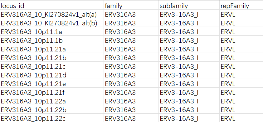
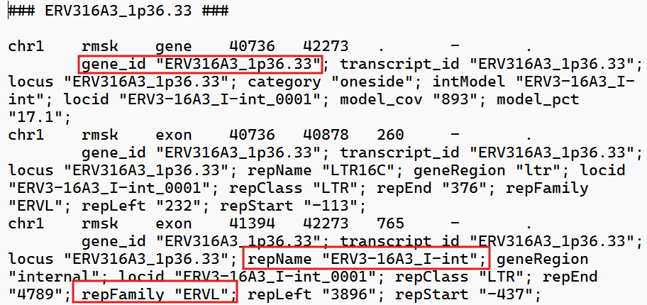
gtf文件:
各列含义:
locus_id:计数直接得到的feature名,对应gtf中的gene_idrepFamily:gtf中的repFamily,应该是超家族/大类,只有ERVK/ERVL/ERV1这三种-
subfamily:gtf中的intModel/repName,其中以gene行的intModel优先(如果这个位点在GTF的gene记录里有intModel,就认为它是该位点最核心、最想表达的“内部模型/亚家族标签”,从上面的截图中可以看到,有时一个位点还会有LTR的标记,不过由于计数结果中并没有标明某个读段到底是ltr还是int,就统一都拿int的名字来指代了。如果没有int就用LTR名称在处理时,因为它们都以
-int结尾(表示internal模块),为了更美观将其去掉,只保留前面的家族名 -
family:使用上次的方法,直接从feature名中以-为分隔截取的经过对比,其实subfamily和前面直接按
-分隔的结果差不多,主要的区别是有些subfamily的名称不一致,比如HML1在这次的聚合方法中变成了HERVK14(HMLx->HERVKx)
最终得到的family/subfamily名:
ERV3-16A3_I ERVL-B4     ERVL-E      ERVL
Harlequin   HERV30      HERV3       HERV4_I
HERV9       HERVE_a     HERVE       HERV-Fc1
HERV-Fc2    HERVFH19    HERVFH21    MER50
HERVH48     HERVH       HERVIP10FH  HERVIP10F
HERVI       HERVK11D    HERVK11     HERVK14C
HERVKC4     HERVL18     HERVL32     HERVL40
HERVL66     HERVL74     HERVL       HERVP71A
HERVS71     HERV17      HERVK14     HERVK
HERVK9      HERVK13     HERVK22     HERVK3
HUERS-P1    HUERS-P2    HUERS-P3b   HUERS-P3
LTR19       LTR23       LTR25       LTR46
LTR57       MER101      MER34B      MER41
MER4B       MER4        MER61       PABL_A
PABL_B      PRIMA41     PRIMA4      PRIMAX
我还找了当时用featureCounts得到的结果,其实家族名也都是
HERV16   HERV9N     HERVIP10F  HERVL    HERVK13
HERVL40  HERVH      HERVL66    HERVFH21 HERV9
HERVFH19 HERVIP10FH HERVK      HERV3    HERVE
HERV9NC  HERVL74    HERV       HERV35I  HERVK14C
HERV1    HERV4      HERVK22    HERV30   HERVS71
HERVK11  HERV17     HERVIP10B3 HERVK14  HERVL18
HERVP71A HERVL32    HERVH48    HERVKC4  HERVI
HERVK3   HERVK11D   HERV15     HERVK9
这种,没有特别标准的HERVK/HERVH/HERVL……这种聚合(featureCounts用的是repeatmasker官网下载的gtf,我自己提取了名字以HERV开头的行,这里我用的stellarscope作者自己整理的gtf,会包含一些ltr以及一些看起来不像HERV的条目)
一个问题:subfamily看起来很杂乱,repfamily又只有这三类,有没有一个中间层级?
- 在ucsc中搜索subfamily:PRIMA4-int的示例结果,其中的family似乎就是ERV1
- 在dfam中搜索subfamily:HERVE的示例结果,注意description那一栏,ERV1后直接就是不同的subfamily了。而结果中
PABL_B-int这种名字不包括HERVE的,能被搜索出来是因为 点进去之后的summary中提到与HERVE相关(“This is related to the HERV3/HERV4/HERVE group of ERVs”/”it was probably dependent on HERVE_a”),但也没有提到归属关系 - 而gtf文件中更没有相关记述,所以就难以找到中间层级,因此我只能试着去掉后缀(
-a/-A这些),并按前缀聚合,不过因为这个是没有依据的,所以后面我也不太想用这个层级
ERV3-16A3 ERVL      Harlequin HERV30    HERV3
HERV4     HERV9     HERVE     HERV-Fc   HERVFH
MER50     HERVH     HERVIP10F HERVI     HERVK
HERVL     HERVP71A  HERVS71   HERV17    HUERS
LTR19     LTR23     LTR25     LTR46     LTR57
MER101    MER34B    MER41     MER4B     MER4
MER61     PABL      PRIMA
替换原assay
注:因为前面构建映射时没有把--no-feature这个feature写进去,所以后面聚合时,会自动把这个过滤掉,而hERV位点的assay是直接用原始计数矩阵导入的,因此nCount_HERV和nCount_HERV_family不同
# meta信息
metadata_xlsx <- "/public/home/GENE_proc/wth/GSE157827/raw_data/metadata/metadata.xlsx"
sample_info_xlsx <- "/public/home/GENE_proc/wth/GSE157827/raw_data/metadata/sample_info.xlsx"
meta_map <- readxl::read_xlsx(metadata_xlsx)
sample_info <- readxl::read_xlsx(sample_info_xlsx)
meta_map <- meta_map |> select(individuals, srr_id, sample_id, tissue)
colnames(meta_map) <- c("sample_id","SRR_id","GSM","tissue")
metadata <- meta_map |> left_join(sample_info, by="sample_id")
gsm2sample <- metadata |> distinct(GSM, sample_id)
# 读取计数矩阵
data_root <- "/public/home/GENE_proc/wth/GSE157827/mtx"
seu <- readRDS("/public/home/GENE_proc/wth/GSE157827/my_data/GSE157827_celltype.rds")
normalize_barcode <- function(x) {
  ifelse(grepl("-\\d+$", x), x, paste0(x, "-1"))
}
read_one_gsm_herv_new <- function(GSM){
  herv_dir <- file.path(data_root, GSM, "hERV_new")  # 这里是你要的新文件夹名
  mat <- ReadMtx(
    mtx      = file.path(herv_dir, "counts.mtx"),
    features = file.path(herv_dir, "features.tsv"),
    cells    = file.path(herv_dir, "barcodes.tsv"),
    feature.column = 1
  )
  sample_name <- gsm2sample$sample_id[gsm2sample$GSM == GSM][1]
  colnames(mat) <- paste(GSM, sample_name, normalize_barcode(colnames(mat)), sep = "_")
  mat
}
gsm_ids <- unique(seu$GSM)
herv_list <- lapply(gsm_ids, read_one_gsm_herv_new)
herv_counts_new <- do.call(cbind, herv_list)
# 家族级聚合
herv_map <- read.csv("/public/home/GENE_proc/wth/GSE157827/raw_data/metadata/hERV_locus2family.csv")
aggregate_herv_counts <- function(herv_counts, map, group_by = c("family","subfamily","repFamily", "family_new")) {
  group_by <- match.arg(group_by)
  keep_loci <- intersect(rownames(herv_counts), map$locus_id)
  map2 <- map[match(keep_loci, map$locus_id), ]
  map2 <- map2[!is.na(map2[[group_by]]) & nzchar(map2[[group_by]]), ]
  mat <- herv_counts[map2$locus_id, , drop = FALSE]
  grp <- map2[[group_by]]
  f <- factor(grp, levels = unique(grp))
  G <- sparseMatrix(
    i = seq_along(f),
    j = as.integer(f),
    x = 1,
    dims = c(length(f), nlevels(f)),
    dimnames = list(rownames(mat), levels(f))
  )
  out <- Matrix::t(G) %*% mat
  out
}
herv_family_counts_new <- aggregate_herv_counts(herv_counts_new, herv_map, group_by = "subfamily")
herv_repfamily_counts_new <- aggregate_herv_counts(herv_counts_new, herv_map, group_by = "repFamily")
herv_family_new_counts_new <- aggregate_herv_counts(herv_counts_new, herv_map, group_by = "family_new")
# 将新计数矩阵的细胞与原来的对齐
align_to_cells <- function(mat, cells){
  mat <- mat[, cells, drop = FALSE]
  mat
}
cells <- colnames(seu)
herv_counts_new  <- align_to_cells(herv_counts_new, cells)
herv_family_counts_new <- align_to_cells(herv_family_counts_new, cells)
herv_repfamily_counts_new <- align_to_cells(herv_repfamily_counts_new, cells)
herv_family_new_counts_new <- align_to_cells(herv_family_new_counts_new, cells)
# 替换原assay
replace_assay <- function(seu, assay_name, counts){
  counts <- as(counts, "dgCMatrix")
  seu[[assay_name]] <- CreateAssayObject(counts = counts)
  seu
}
seu <- replace_assay(seu, "HERV", herv_counts_new)
seu <- replace_assay(seu, "HERV_family", herv_family_counts_new)
seu <- replace_assay(seu, "HERV_repfamily", herv_repfamily_counts_new)
seu <- replace_assay(seu, "HERV_family_new", herv_family_new_counts_new)
# 更新metadata
herv_counts <- GetAssayData(seu, assay="HERV", slot="counts")
rna_counts  <- GetAssayData(seu, assay="RNA",  slot="counts")
seu$nCount_HERV   <- Matrix::colSums(herv_counts)
seu$nFeature_HERV <- Matrix::colSums(herv_counts > 0)
seu$nCount_HERV_family   <- Matrix::colSums(GetAssayData(seu, assay="HERV_family", slot="counts"))
seu$nFeature_HERV_family <- Matrix::colSums(GetAssayData(seu, assay="HERV_family", slot="counts") > 0)
seu$HERV_fraction <- seu$nCount_HERV / Matrix::colSums(rna_counts)
# 标准化
normalize_herv_by_rna_depth <- function(seu, assay, scale.factor = 10000) {
  rna_counts  <- GetAssayData(seu, assay = "RNA",  slot = "counts")
  herv_counts <- GetAssayData(seu, assay = assay, slot = "counts")
  lib_rna <- Matrix::colSums(rna_counts)
  herv_norm <- t(t(herv_counts) / lib_rna) * scale.factor
  herv_norm@x <- log1p(herv_norm@x)
  seu <- SetAssayData(seu, assay = assay, slot = "data", new.data = herv_norm)
  return(seu)
}
seu <- normalize_herv_by_rna_depth(seu, "HERV")
seu <- normalize_herv_by_rna_depth(seu, "HERV_family")
seu <- normalize_herv_by_rna_depth(seu, "HERV_repfamily")
seu <- normalize_herv_by_rna_depth(seu, "HERV_family_new")
# 保存数据
DefaultAssay(seu) <- "RNA"
saveRDS(
    seu,
    file = "/public/home/GENE_proc/wth/GSE157827/my_data/GSE157827_celltype_new.rds",
    compress = "xz"
)
共包含5个assay:
RNA:普通基因(STAR的输出)HERV:hERV位点级计数(stellarscope的输出)HERV_family:subfamily级计数(根据gtf文件)HERV_family_new:family级计数(根据前缀合并到更大的层级)HERV_repfamily:超家族/class级计数(根据gtf文件)
step1:总体/超家族重调情况
总体思路:
- 把所有hERV位点的计数加在一起
- 从原始count开始累加
- 用RNA库深度标准化
- 把累加后的结果作为一个新feature
HERV-total保存在HERV_repfamily里
- AD-NC的差异分析:沿用之前的思路——
FindMarkers+test.use="MAST"+latent.vars=c("orig.ident","nCount_RNA","percent_mito")- 所有细胞
- 取出各细胞类型的细胞单独做
因为在之前的分析中,我看到hERV-low(偏向AD的细胞)普遍测序深度较低,先看看AD/NC的测序深度有没有显著差别
meta <- seu@meta.data %>%
  filter(!is.na(group), !is.na(nCount_RNA), !is.na(celltype)) %>%
  mutate(group = factor(group, levels = c("NC","AD")))
# 全体细胞
p1 <- ggplot(meta, aes(x = group, y = nCount_RNA)) +
  geom_violin(scale = "width", trim = TRUE) +
  stat_compare_means(method = "t.test", label = "p.signif") +
  scale_y_log10()
# 各大细胞类型
p2 <- ggplot(meta, aes(x = celltype, y = nCount_RNA, fill = group)) +
  geom_violin(scale = "width", trim = TRUE, position = position_dodge(width = 0.9)) +
  stat_compare_means(method = "t.test", label = "p.signif") +
  scale_y_log10()
p1 | p2
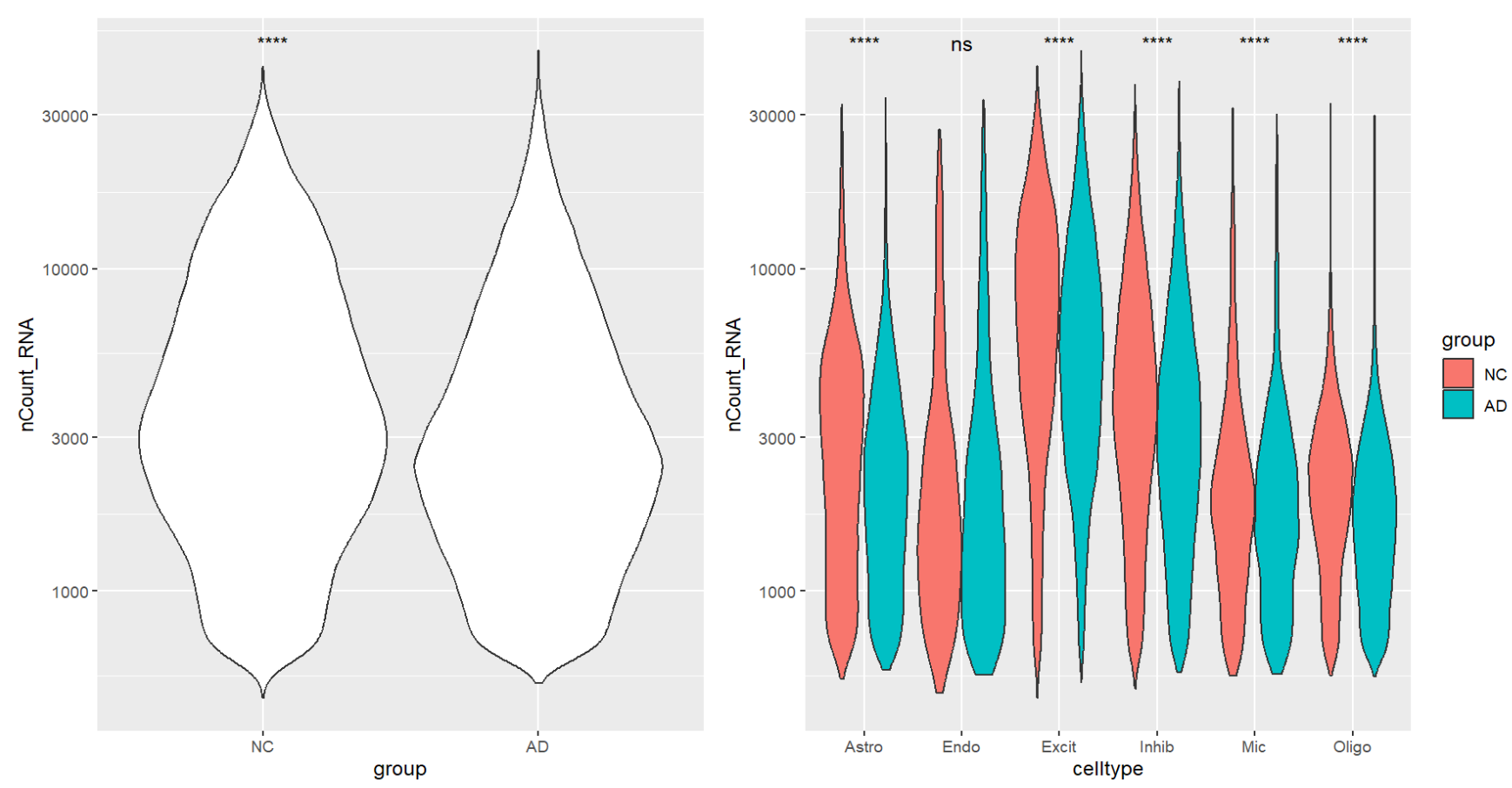
看起来AD的nCount_RNA平均更低,也许前面得到的“AD中hERV表达量更低”的结论是受了测序深度的影响,所以后面尽力用协变量消除一下测序深度的影响吧
- 不过测序深度低是会导致hERV标准化后的值变高还是变低,这个还不太确定,因为我们标准化的方法是
HERV_count / RNA_lib,是count变少的多,还是RNA_lib变少的多
获得总hERV计数:
# hERV计数矩阵
herv_counts <- GetAssayData(seu, assay = "HERV_repfamily", slot = "counts")
herv_total_counts <- Matrix::colSums(herv_counts)
# RNA库深度
rna_counts <- GetAssayData(seu, assay = "RNA", slot = "counts")
rna_lib <- Matrix::colSums(rna_counts)
# 标准化
sf <- 1e4
herv_total_data <- log1p((herv_total_counts / rna_lib) * sf)
# 写入一个新assay
new_counts_row <- Matrix::Matrix(herv_total_counts, nrow = 1, sparse = TRUE)
rownames(new_counts_row) <- "HERV_total"
colnames(new_counts_row) <- colnames(seu)
new_data_row <- Matrix::Matrix(herv_total_data, nrow = 1, sparse = TRUE)
rownames(new_data_row) <- "HERV_total"
colnames(new_data_row) <- colnames(seu)
# 添加到HERV_repfamily的assay中
mat_counts <- GetAssayData(seu, assay = "HERV_repfamily", slot = "counts")
mat_counts2 <- rbind(mat_counts, new_counts_row)
mat_data <- GetAssayData(seu, assay = "HERV_repfamily", slot = "data")
mat_data2 <- rbind(mat_data, new_data_row)
new_assay <- CreateAssayObject(counts = mat_counts2)
new_assay <- SetAssayData(new_assay, slot="data", new.data = mat_data2)
seu[["HERV_repfamily"]] <- new_assay
# 准备差异分析
Idents(seu) <- factor(seu$group, levels = c("NC","AD"))
DefaultAssay(seu) <- "HERV_repfamily"
latent <- c("orig.ident", "nCount_RNA", "percent_mito")
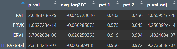
全体细胞:
res_all <- FindMarkers(
object = seu,
ident.1 = "AD", ident.2 = "NC",
test.use = "MAST",
latent.vars = latent,
logfc.threshold = 0, min.pct = 0, return.thresh = 1
)
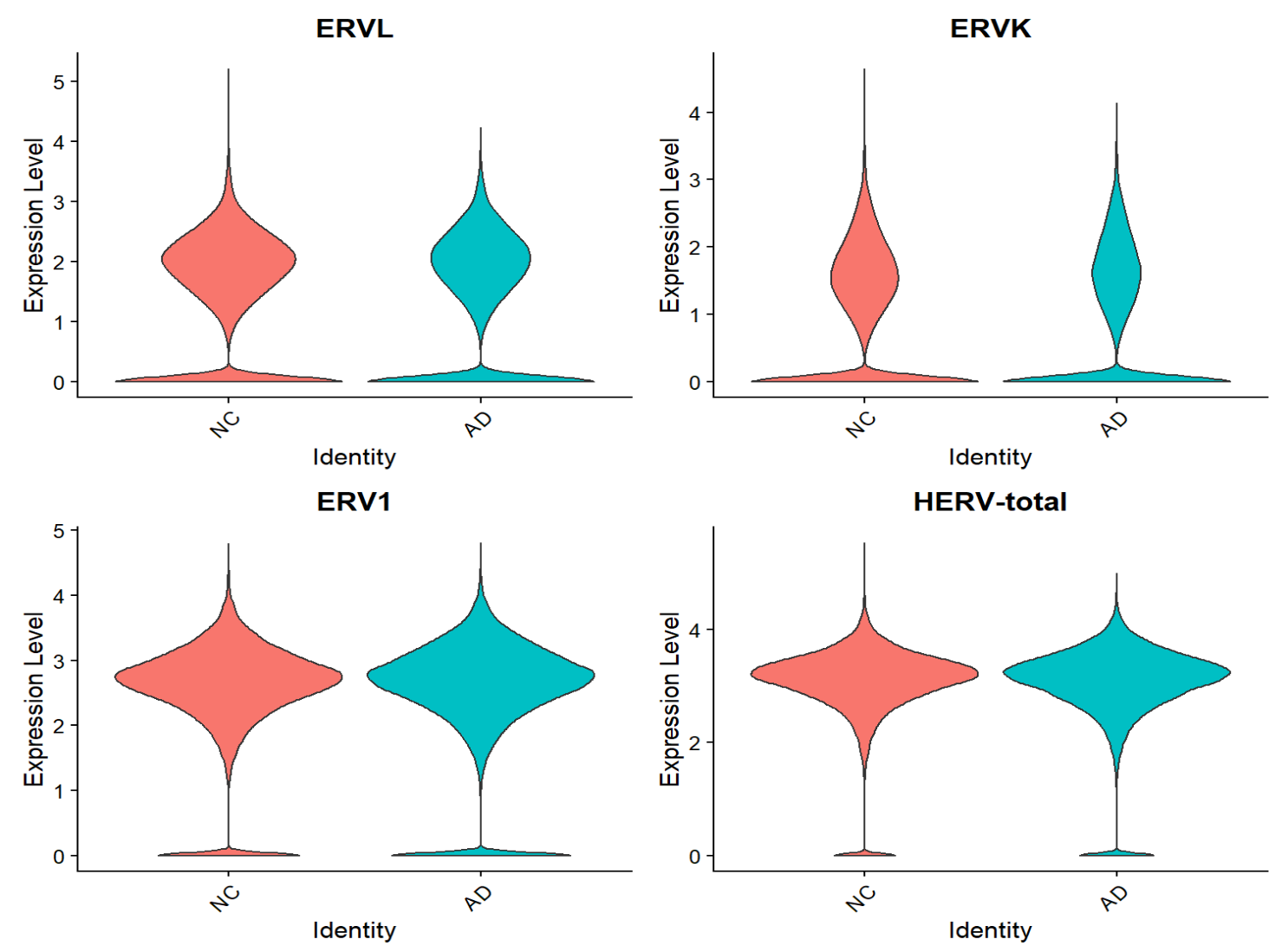
VlnPlot(seu, features = Features(seu), group.by = "group", pt.size = 0, ncol = 2)
各细胞类型:
celltypes <- sort(unique(seu$celltype))
run_one_ct <- function(ct) {
obj <- subset(seu, subset = celltype == ct)
n_tab <- table(obj$group)
print(paste("running:", ct))
fm <- FindMarkers(
object = obj,
ident.1 = "AD", ident.2 = "NC",
test.use = "MAST",
latent.vars = latent,
logfc.threshold = 0, min.pct = 0, return.thresh = 1
)
out <- fm %>%
tibble::rownames_to_column("feature") %>%
mutate(celltype = ct,
n_NC = unname(n_tab["NC"]),
n_AD = unname(n_tab["AD"]))
out
}
res_by_ct <- do.call(rbind, lapply(celltypes, run_one_ct))
# 只看p值<0.05的
View(res_by_ct %>%
dplyr::filter(p_val_adj<0.05) %>%
arrange(p_val_adj) %>%
select(celltype, n_NC, n_AD, avg_log2FC, p_val, p_val_adj, everything()))
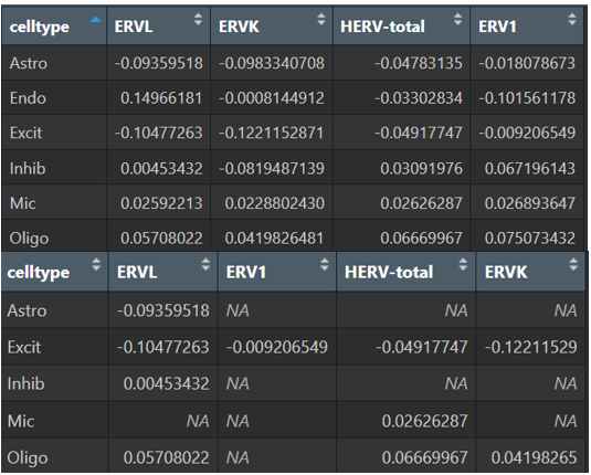
# 全部数据的logFC
View(
res_by_ct %>%
select(celltype, avg_log2FC, feature) %>%
tidyr::pivot_wider(id_cols = celltype, names_from = feature, values_from = avg_log2FC)
)
# 过滤p值后的logFC
View(
res_by_ct %>%
dplyr::filter(p_val_adj<0.05) %>%
select(celltype, avg_log2FC, feature) %>%
tidyr::pivot_wider(id_cols = celltype, names_from = feature, values_from = avg_log2FC,)
)
VlnPlot(seu, features = Features(seu), group.by = "celltype", split.by = "group", pt.size = 0, ncol = 2) +
RotatedAxis()
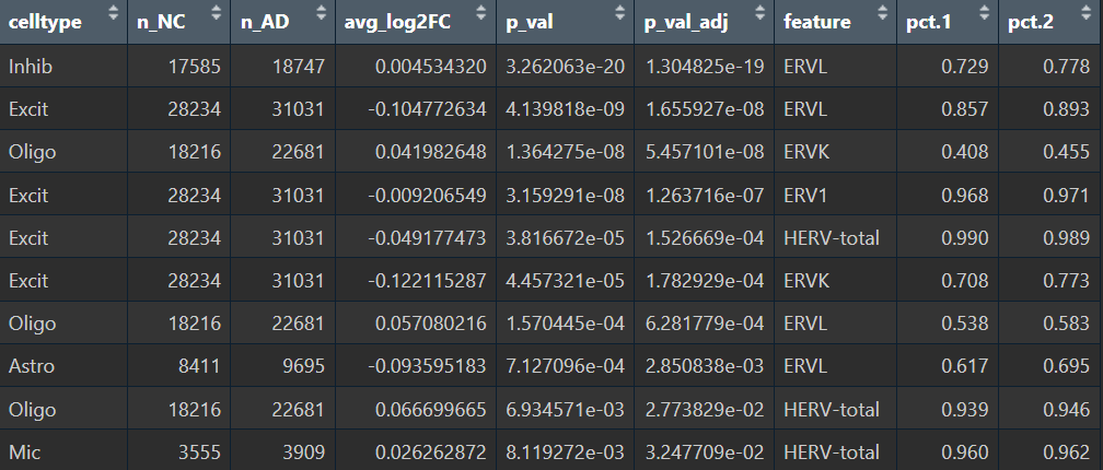
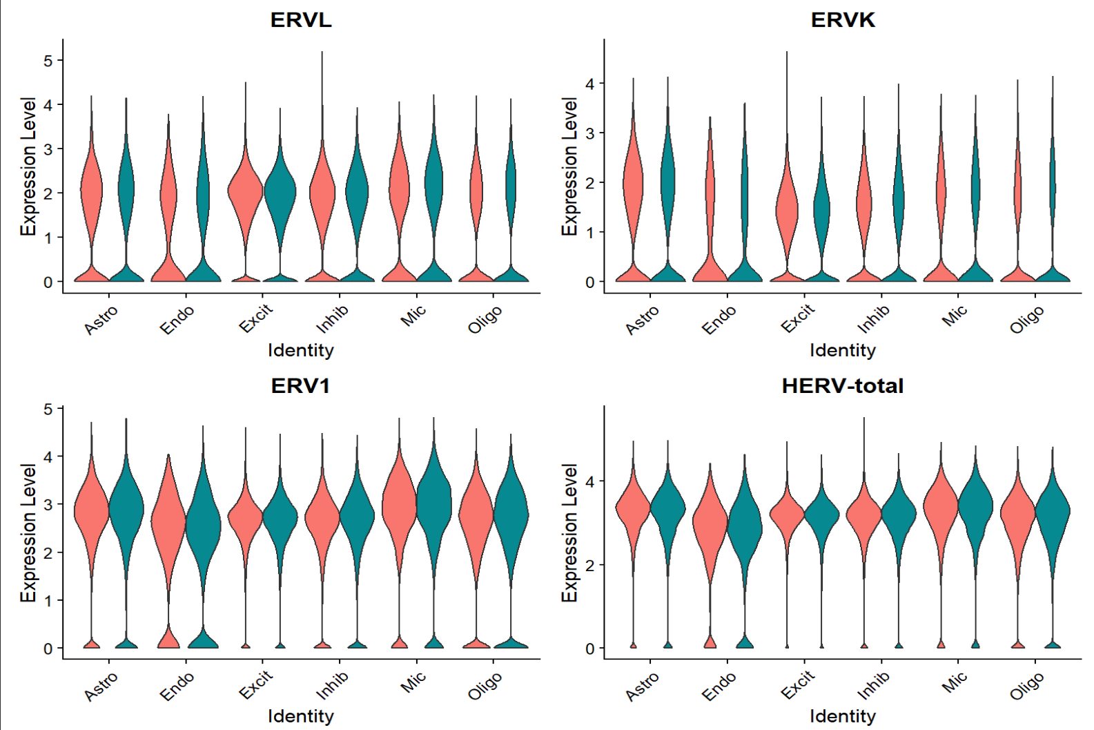
综上,hERV总体在全体细胞中并没有特别明显的重调(RVL/ERVK略低、ERV1略高,但效应量极小),如果按细胞类型拆开:
- Excit(兴奋性神经元):一致下调,且logFC相对较大
- Oligo(少突胶质细胞):一致上调
- Astro(星形胶质细胞):ERVL下调
- Mic(小胶质细胞):total轻微上升
- 其它细胞效应都较小,或由于细胞数过少而导致padj较大
找了一些与HERV AD相关的文献,不过都是RNA-seq的