snRNA-Seq的fastq数据分析
other-other2025.12.03-2025.12.17研究进展
scRNA-seq的测序数据
对于普通的RNA-seq双端测序,是把一段DNA两段接上接头,固定一端后从一头往里读,之后再翻过去从另一头往里读,最后fastq有两份,这个R1/R2是从同一片段两端读进来的序列,内容通常是对称的,所以处理时不需要进行区分
在scRNA-seq中,我需要知道两件事:
- “这是哪个细胞的转录本”——细胞条形码(cell barcode, CB):构建基因×细胞的文库,要知道哪些reads来自同一个细胞。条形码根据建库方法有所不同,10X Genomics通常是一个16bp的条形码,SPLiT-seq/Parse共有3个index,每个8bp,最后拼成24bp的条形码。最后所有来自这个细胞的转录本,在建库时都会带上这一段序列,比对和计数时就通过条形码把reads按细胞分组
- “这几条read是不是同一个原始分子PCR放大出来的”——UMI(unique molecular identifier):如果某个mRNA只有1个分子,但PCR放大了1000倍,就会测到1000条reads,如果直接按reads数当表达量,就会被PCR偏好性影响。于是在每个原始分子(转录本)上随机加一个UMI(通常10bp),无论PCR怎么放大,UMI不会变,最后统计时,“同一细胞、同一基因、同一个UMI”就只算一个分子
在scRNA-seq的文库构建时,CB/UMI被特意设计在某一端的固定位置,这样双端测序结果中,就会有一端是CB/UMI,另一端才是真正的cDNA序列。比如10x Genomics的R1是16bp的CB+10bp的UMI+后面的linker,R2是cDNA序列,Parse Evercode/SPLiT-seq的R1是cDNA,R2是UMI+多组CB
- cDNA的每条读段,前面有一段高度保守的motif(接头),后面序列多样(真正的基因序列)
- UMI+CB的每条读段,UMI段多样性搞,UMI-CB或CB-后面序列中间有高度保守的linker,CB段序列结构固定,通常只能是在有固定数量的序列库(whitelist)中选取
在STARsolo/cellranger等单细胞比对/计数软件中,需要先告诉它哪端是cDNA/CB+UMI,并指出UMI和CB的位置坐标
- 对于每个cDNA序列,就像普通RNA-seq一样比对到参考基因组上,并判断这个read落在哪个基因
- 对于每个UMI+CB序列,会根据坐标切出UMI+CB(如果有多段CB,就会把这些CB按顺序拼起来当作一个整体),之后根据whitelist做纠错/过滤(可选)。以上信息都会保存在BAM文件中
- 从BAM中获取CB/UMI和比对信息,丢掉mapping质量低、不在基因上的read。在每个
(cell, gene)里,把UMI去重(“同一细胞、同一基因、同一个UMI”只算一次),聚合得到一个counts[gene, cell] - 最后得到:
-
matrix.mtx:稀疏矩阵(行=基因,列=细胞) -
barcodes.tsv:每一列对应的CB -
features.tsv:每一行对应的基因名
-
数据下载和建索引
由telescope的同作者开发的针对单细胞数据的hERV位点级分析工具Stellarscope
先跟着官方教程走一遍
- 发现官方教程有个25G的文件,其下载速度只有200K不到,没法用
- 直接用咱的fastq数据
构建STAR索引:
- 人类基因组GRCh38.p14.genome.fa.gz
- 人类基因组注释gencode.v49.annotation.gtf.gz
- hERV专用注释HERV_rmsk.hg38.v2
cd /public/home/wangtianhao/Desktop/STAR_ref/
module load miniconda3/base
conda activate STAR
STAR \
  --runThreadN 16 \
  --runMode genomeGenerate \
  --genomeDir hg38 \
  --genomeFastaFiles GRCh38.p14.genome.fa \
  --sjdbGTFfile gencode.v49.annotation.gtf
注:建索引以及之后比对时都不需要hERV注释,其实连人类基因组注释都可以不用,这个gtf只是为了识别splice junction,STAR比对时不需要知道哪些位置是HERV
下载数据:
cd /public/home/wangtianhao/Desktop/GSE233208/1204test/fastq/
module load miniconda3/base
conda activate fastq-download
nohup parallel-fastq-dump --sra-id SRR24710599 --threads 8 --split-files --tmpdir ./fastq_temp --gzip &
# 或者
nohup axel -n 8 ftp://ftp.sra.ebi.ac.uk/vol1/fastq/SRR247/098/SRR24710598/SRR24710598_2.fastq.gz > /dev/null 2> error.log &
nohup axel -n 8 ftp://ftp.sra.ebi.ac.uk/vol1/fastq/SRR247/098/SRR24710598/SRR24710598_1.fastq.gz > /dev/null 2> error.log &
SRA run上显示Bytes为17.56G的gz下载下来得到双端共190G的fastq,Bytes为18.51G的gz下载下来得到双端共23.4G的fastq.gz(下载时间差不多,都在6h左右)
质控:以下列举的质控好像只是生成质量报告,并不实际修改读段(而且不是专门给scRNA-seq设置的),了解即可,后续没有用
cd /public/home/wangtianhao/Desktop/GSE233208/1204test/
mkdir -p qc
module load miniconda3/base
conda activate fastqc
fastqc fastq/*.fastq.gz -o qc
cd qc
multiqc .
自动下载:先建一个SRR_Acc_List.txt,里面放上要下载的SRR号(从SRA run界面的Accession List按钮下载)
cd /public/home/wangtianhao/Desktop/GSE233208/fastq
module load miniconda3/base
conda activate fastq-download
for SRR in $(cat SRR_Acc_List.txt); do
    parallel-fastq-dump --sra-id ${SRR} --tmpdir ./fastq_temp --threads 8 --split-files --gzip
done
GSE138852
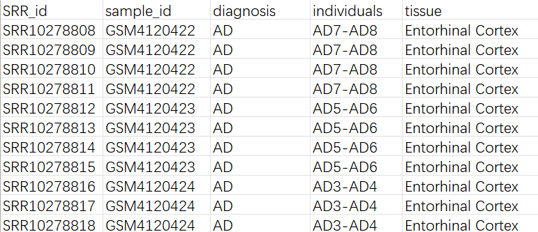
数据量较小(共78.18G,碱基数153.78G,样本量8个),但作者提供了详细的计数矩阵+条形码+基因(包括每个SRR run的和总的),并且使用10X Genomics,条形码和UMI位置易确定,打算先用这个数据集跑通基本pipeline(STARsolo+stellarscope+构建Seurat对象)
点开其中一个样本的页面GSM4120422,可以看到是用什么测序技术测的(UMI和BC的位置和长度),关键信息:
I1 read: contains the sample index.
R1 read: contains the cell barcode (first 16 nt) and UMI (next 10 nt).
R2 read: contains the RNA sequence.
Using the Grch38 (1.2.0) reference from 10x Genomics
using the Chromium Single Cell 3′ Library & Gel Bead Kit v2 (10X Genomics, #PN-120237)
进入SRA run中下载
STAR比对
因为下载下来得到的是SRRxxx_1.fastq.gz/SRRxxx_2.fastq.gz/SRRxxx_3.fastq.gz这样的文件,首先检测哪个是cDNA,哪个是UMI+barcode
zcat SRR10278808_1.fastq.gz | awk 'NR%4==2 {print length($0)}' | head
zcat SRR10278808_2.fastq.gz | awk 'NR%4==2 {print length($0)}' | head
zcat SRR10278808_3.fastq.gz | awk 'NR%4==2 {print length($0)}' | head
-
SRRxxx_1.fastq.gz:8bp——index,对STAR计数不重要,可忽略 -
SRRxxx_2.fastq.gz:26bp——UMI+barcodes -
SRRxxx_3.fastq.gz:116bp——cDNA
whitelist从哪里下载:有时CellRanger的安装目录里就有,不过我没找到,直接到GitHub的开源项目中搜,比如10X Cell Ranger whitelists,把两个txt解压即可。因为是v2版本,所以用737K-august-2016.txt
cd /public/home/wangtianhao/Desktop/GSE138852/
module load miniconda3/base
conda activate STAR
mkdir -p star/res
cd star
# 注意以下命令执行时删掉#的行,否则只读到第一个#就不往下读了
STAR \
  --runMode alignReads \
  --runThreadN 16 \
  --genomeDir /public/home/wangtianhao/Desktop/STAR_ref/hg38/ \
  --readFilesIn /public/home/wangtianhao/Desktop/GSE138852/fastq/SRR10278808_3.fastq.gz /public/home/wangtianhao/Desktop/GSE138852/fastq/SRR10278808_2.fastq.gz \
  --readFilesCommand zcat \
  --outFileNamePrefix res/SRR10278808_ \
  # 条形码 \
  --soloType CB_UMI_Simple \
  --soloCBstart 1 \
  --soloCBlen 16 \
  --soloUMIstart 17 \
  --soloUMIlen 10 \
  --soloBarcodeReadLength 0 \
  --soloCBwhitelist /public/home/wangtianhao/Desktop/STAR_ref/whitelist/737K-august-2016.txt \
  # 计数/细胞筛选设置 \
  --clipAdapterType CellRanger4 \
  --soloCBmatchWLtype 1MM_multi_Nbase_pseudocounts \
  --soloUMIfiltering MultiGeneUMI_CR \
  --soloUMIdedup 1MM_CR \
  # BAM输出和Tags(给Stellarscope用) \
  --outSAMtype BAM SortedByCoordinate \
  --outSAMattributes NH HI nM AS CR UR CB UB GX GN sS sQ sM \
  # Stellarscope要求保留多重比对 \
  --outSAMunmapped Within \
  --outFilterScoreMin 30 \
  --limitOutSJcollapsed 5000000 \
  --outFilterMultimapNmax 500 \
  --outFilterMultimapScoreRange 5
stellarscope计数
module load miniconda3/base
conda activate stellarscope
cd /public/home/wangtianhao/Desktop/GSE138852/stellarscope/
mkdir -p res
# 按名称排序
samtools view -@1 -u -F 4 -D CB:<(tail -n+1 /public/home/wangtianhao/Desktop/GSE138852/star/res/SRR10278808_Solo.out/Gene/filtered/barcodes.tsv) /public/home/wangtianhao/Desktop/GSE138852/star/res/SRR10278808_Aligned.sortedByCoord.out.bam | samtools sort -@16 -n -t CB -T ./tmp > ./res/Aligned.sortedByCB.bam
# 计数
stellarscope assign \
  --exp_tag SRR10278808 \
  --outdir /public/home/wangtianhao/Desktop/GSE138852/stellarscope/res \
  --nproc 16 \
  --stranded_mode F \
  --whitelist /public/home/wangtianhao/Desktop/GSE138852/star/res/SRR10278808_Solo.out/Gene/filtered/barcodes.tsv \
  --pooling_mode individual \
  --reassign_mode best_exclude \
  --max_iter 500 \
  --updated_sam \
  /public/home/wangtianhao/Desktop/GSE138852/stellarscope/res/Aligned.sortedByCB.bam \
  /public/home/wangtianhao/Desktop/STAR_ref/transcripts.gtf
循环运行并构建Seurat对象
总体思路:普通基因使用STARsolo计数,hERV使用stellarscope计数,而最终我们是用普通基因先构建Seurat对象,再把stellarscope计数得到的矩阵作为一个assay挂载上去
workDir=/public/home/GENE_proc/wth/GSE138852/
genomeDir=/public/home/wangtianhao/Desktop/STAR_ref/hg38/
whitelist=/public/home/wangtianhao/Desktop/STAR_ref/whitelist/737K-august-2016.txt
hERV_gtf=/public/home/wangtianhao/Desktop/STAR_ref/transcripts.gtf
res_barcodes=barcodes
res_features=features
res_counts=counts
# STARsolo + stellarscope
cd ${workDir}
module load miniconda3/base
for SRR in $(cat ./fastq/SRR_Acc_List.txt); do
  conda activate STAR
  mkdir -p star
  STAR \
    --runMode alignReads \
    --runThreadN 16 \
    --genomeDir ${genomeDir} \
    --readFilesIn ./fastq/${SRR}_3.fastq.gz ./fastq/${SRR}_2.fastq.gz \
    --readFilesCommand zcat \
    --outFileNamePrefix star/${SRR}_ \
    --soloType CB_UMI_Simple \
    --soloCBstart 1 \
    --soloCBlen 16 \
    --soloUMIstart 17 \
    --soloUMIlen 10 \
    --soloBarcodeReadLength 0 \
    --soloCBwhitelist ${whitelist} \
    --clipAdapterType CellRanger4 \
    --soloCBmatchWLtype 1MM_multi_Nbase_pseudocounts \
    --soloUMIfiltering MultiGeneUMI_CR \
    --soloUMIdedup 1MM_CR \
    --outSAMtype BAM SortedByCoordinate \
    --outSAMattributes NH HI nM AS CR UR CB UB GX GN sS sQ sM \
    --outSAMunmapped Within \
    --outFilterScoreMin 30 \
    --limitOutSJcollapsed 5000000 \
    --outFilterMultimapNmax 500 \
    --outFilterMultimapScoreRange 5
  conda deactivate
  conda activate stellarscope
  mkdir -p stellarscope/${SRR}
  samtools view -@1 -u -F 4 -D CB:<(tail -n+1 ./star/${SRR}_Solo.out/Gene/filtered/barcodes.tsv) ./star/${SRR}_Aligned.sortedByCoord.out.bam | samtools sort -@16 -n -t CB -T ./tmp > ./stellarscope/${SRR}/Aligned.sortedByCB.bam
  stellarscope assign \
    --outdir ./stellarscope/${SRR} \
    --nproc 16 \
    --stranded_mode F \
    --whitelist ./star/${SRR}_Solo.out/Gene/filtered/barcodes.tsv \
    --pooling_mode individual \
    --reassign_mode best_exclude \
    --max_iter 500 \
    --updated_sam \
    ./stellarscope/${SRR}/Aligned.sortedByCB.bam \
    ${hERV_gtf}
  conda deactivate
done
# 汇总结果
cd ${workDir}
for SRR in $(cat ./fastq/SRR_Acc_List.txt); do
  mkdir -p mtx/${SRR}/gene
  cp ./star/${SRR}_Solo.out/Gene/filtered/barcodes.tsv ./mtx/${SRR}/gene/${res_barcodes}.tsv
  cp ./star/${SRR}_Solo.out/Gene/filtered/features.tsv ./mtx/${SRR}/gene/${res_features}.tsv
  cp ./star/${SRR}_Solo.out/Gene/filtered/matrix.mtx ./mtx/${SRR}/gene/${res_counts}.mtx
  mkdir -p mtx/${SRR}/hERV
  cp ./stellarscope/${SRR}/stellarscope-barcodes.tsv ./mtx/${SRR}/hERV/${res_barcodes}.tsv
  cp ./stellarscope/${SRR}/stellarscope-features.tsv ./mtx/${SRR}/hERV/${res_features}.tsv
  cp ./stellarscope/${SRR}/stellarscope-TE_counts.mtx ./mtx/${SRR}/hERV/${res_counts}.mtx
done
du -sh ./mtx  # 看看最后的数据有多大--400多M
# tar -czvf mtx.tar.gz ./mtx/
将SRR号和诊断组别等信息整合为一个表格:
从mtx构建Seurat对象:
library(Seurat)
library(Matrix)
library(tidyverse)
library(readxl)
data_root <- "C:\\Users\\17185\\Desktop\\hERV_calc\\GSE138852\\data\\mtx"
metadata_path <- "C:\\Users\\17185\\Desktop\\hERV_calc\\GSE138852\\metadata.xlsx"
# 读取一个SRR,返回一个Seurat对象(普通基因+hERV)
read_one_srr <- function(srr) {
  gene_dir <- file.path(data_root, srr, "gene")
  herv_dir <- file.path(data_root, srr, "hERV")
  # 读取mtx
  gene_counts <- ReadMtx(
    mtx = file.path(gene_dir, "counts.mtx"),
    features = file.path(gene_dir, "features.tsv"),
    cells = file.path(gene_dir, "barcodes.tsv")
  )
  herv_counts <- ReadMtx(
    mtx = file.path(herv_dir, "counts.mtx"),
    features = file.path(herv_dir, "features.tsv"),
    cells = file.path(herv_dir, "barcodes.tsv"),
    feature.column = 1
  )
  # 给不同SRR的细胞加前缀,避免重名
  colnames(gene_counts) <- paste(srr, colnames(gene_counts), sep = "_")
  colnames(herv_counts) <- paste(srr, colnames(herv_counts), sep = "_")
  # 只保留gene和hERV都有的细胞
  common_cells <- intersect(colnames(gene_counts), colnames(herv_counts))
  gene_counts <- gene_counts[, common_cells, drop = FALSE]
  herv_counts <- herv_counts[, common_cells, drop = FALSE]
  # 用普通基因创建Seurat对象
  seu <- CreateSeuratObject(
    counts = gene_counts,
    assay = "RNA",
    project = "AD_hERV"
  )
  # 把hERV作为第二个assay挂上去
  seu[["HERV"]] <- CreateAssayObject(counts = herv_counts)
  # 在metadata里记一下SRR号,后面方便join
  seu$SRR_id <- srr
  return(seu)
}
# 读取metadata
sample_meta <- read_xlsx(metadata_path)
# 列出所有文件夹
srr_ids <- list.dirs(data_root, full.names = FALSE, recursive = FALSE)
# 对所有SRR构建Seurat对象
seu_list <- list()
for (srr in srr_ids) {
  seu <- read_one_srr(srr)
  if (!is.null(seu)) {
    seu_list[[srr]] <- seu
  }
}
# 合并
seu <- Reduce(function(x, y) merge(x, y), seu_list)
rm(seu_list)
head(seu@meta.data)
# 添加metadata
meta_df <- seu@meta.data %>%
  rownames_to_column("cell") %>%
  left_join(sample_meta, by = "SRR_id") %>%
  column_to_rownames("cell")
seu@meta.data <- meta_df
# 合并每个layers
seu <- JoinLayers(seu, assay = "RNA")
# 检查一下layers
Layers(seu, assay = "RNA")
# 保存为rds
saveRDS(
  seu,
  file = "C:\\Users\\17185\\Desktop\\hERV_calc\\GSE138852\\data\\GSE138852.rds",
  compress = "xz"
)
初步验证两个计数矩阵是否正确
基本参数:
seu <- readRDS("C:\\Users\\17185\\Desktop\\hERV_calc\\GSE138852\\data\\GSE138852.rds")
seu[["percent.mt"]] <- PercentageFeatureSet(seu, pattern = "^MT-")
# 维度和细胞名是否对齐
rna_counts  <- GetAssayData(seu, assay = "RNA",  slot = "counts")
herv_counts <- GetAssayData(seu, assay = "HERV", slot = "counts")
dim(rna_counts)
dim(herv_counts)  # 细胞数应该相同
all(colnames(rna_counts) == colnames(herv_counts))  # 细胞名应该相同
# 基本分布
seu$nCount_RNA <- Matrix::colSums(rna_counts)
seu$nFeature_RNA <- Matrix::colSums(rna_counts > 0)
summary(seu$nCount_RNA)
summary(seu$nFeature_RNA)
seu$nCount_HERV <- Matrix::colSums(herv_counts)
seu$nFeature_HERV <- Matrix::colSums(herv_counts > 0)
summary(seu$nCount_HERV)
summary(seu$nFeature_HERV)
# HERV占整个转录本的比例
seu$HERV_fraction <- seu$nCount_HERV / (seu$nCount_HERV + seu$nCount_RNA)
summary(seu$HERV_fraction)
summary(seu$nFeature_RNA)
Min.   :   24
1st Qu.:  187
Median :  256
Mean   :  324
3rd Qu.:  375
Max.   : 3606

summary(seu$nCount_RNA)
Min.   :   88
1st Qu.:  247
Median :  345
Mean   :  458
3rd Qu.:  523
Max.   : 7083
对于经典10x单细胞,每个细胞的基因数nFeature_RNA正常中位数应该在1000-3000左右,每个细胞的UMI数nCount_RNA也应在几千-几万的水平,属于偏低但可以接受的范围,可能是测序深度过低/snRNA-seq的原因
summary(seu$nCount_HERV)
Min.   :  0.0
1st Qu.:  0.0
Median :  2.0
Mean   :  2.4
3rd Qu.:  3.0
Max.   : 48.0

summary(seu$nFeature_HERV)
Min.   :  0.0
1st Qu.:  0.0
Median :  1.0
Mean   :  2.1
3rd Qu.:  3.0
Max.   : 37.0

summary(seu$HERV_fraction)
Min.   :0.000000
1st Qu.:0.000000
Median :0.004149   # 约 0.4%
Mean   :0.005002   # 约 0.5%
3rd Qu.:0.007321   # 约 0.7%
Max.   :0.076271   # 最高~7.6%
理论上,大部分细胞的hERV UMI只有0-几个,feature数也只有0-3个左右,UMI占比没有出现“某些细胞几乎全是HERV,正常基因很少”的情况,符合真实生物信号
画QC图:
seu$QCgroup <- "All_cells"  # 给所有细胞加一个统一分组,防止画图时按SRR分组导致多个柱子的情况
VlnPlot(seu, features = c("nFeature_RNA", "nCount_RNA", "percent.mt"), group.by = "QCgroup", ncol = 3)
FeatureScatter(seu, feature1 = "nCount_RNA", feature2 = "percent.mt", group.by = "QCgroup")
FeatureScatter(seu, feature1 = "nCount_RNA", feature2 = "nFeature_RNA", group.by = "QCgroup")
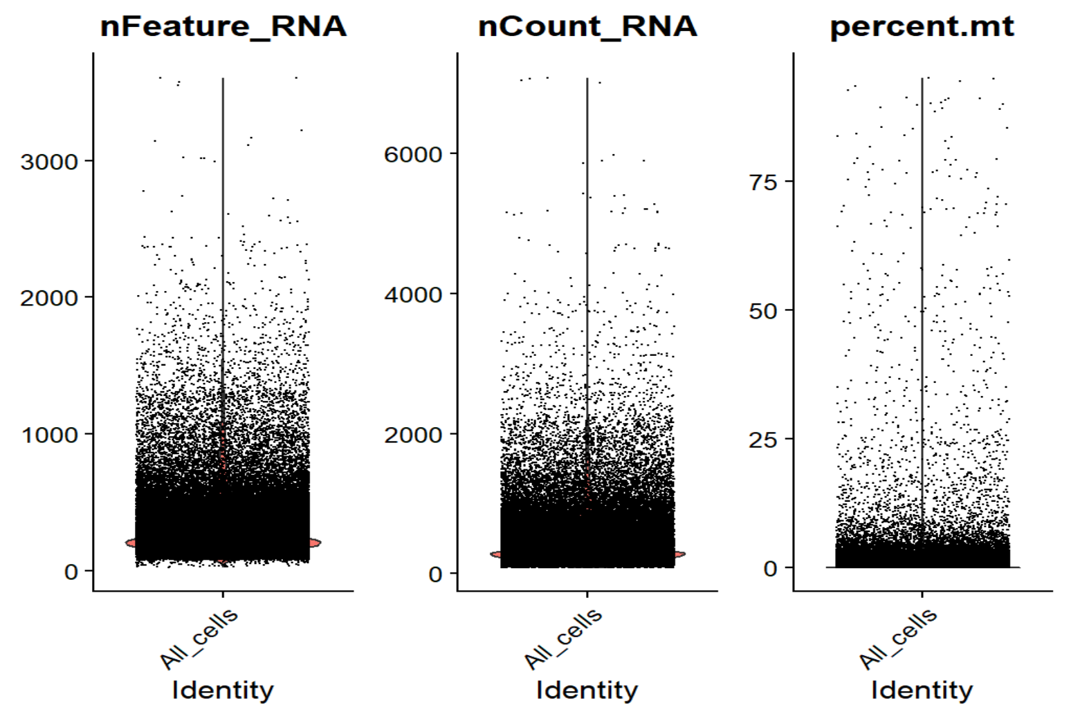
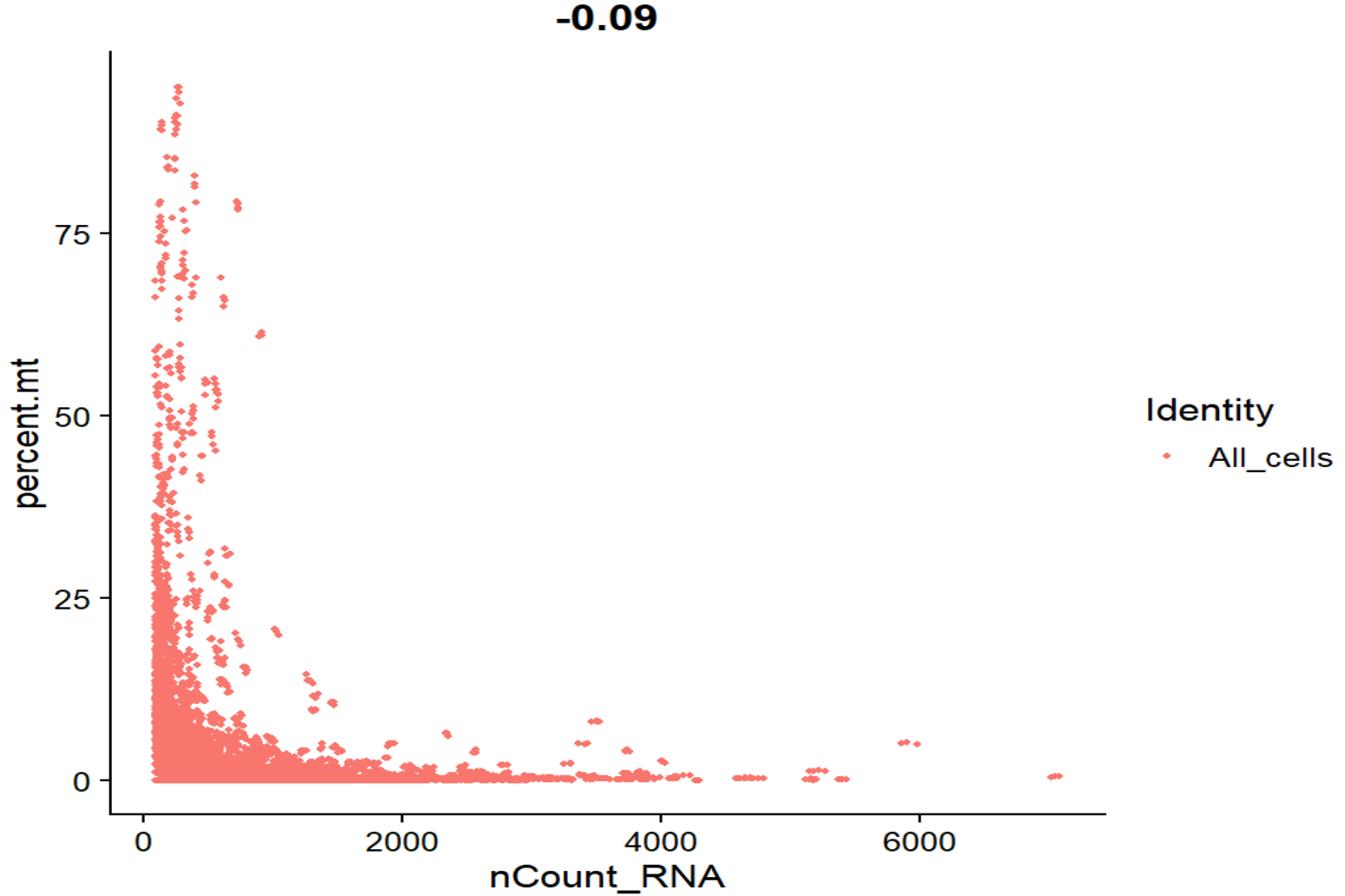
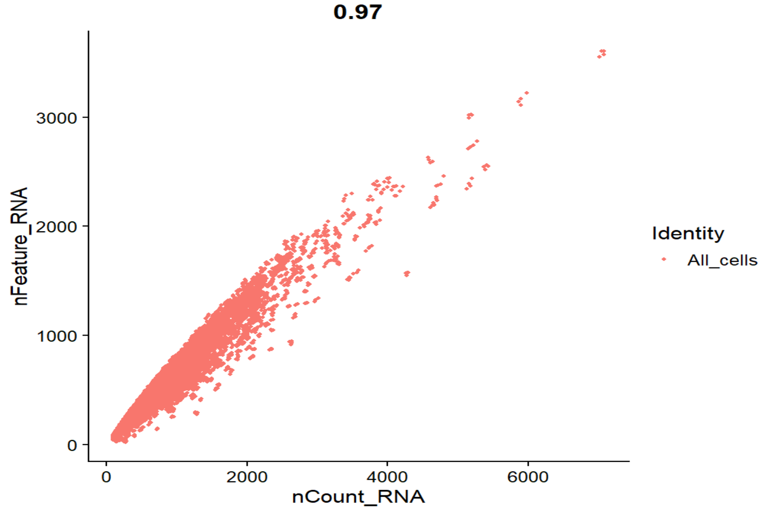
-
nFeature_RNA - nCount_RNA相关系数0.97,整体是一条弯曲的抛物线,没有出现很多“UMI很高但feature很少”的情况 -
nCount_RNA - percent.mt相关系数-0.09,基本接近0,整体是标准的L形,线粒体比例和UMI没有正相关,高线粒体的点主要集中在低UMI端,符合预期
可以据此设置过滤阈值:
seu_qc <- subset(
  seu,
  subset =
    nFeature_RNA > 150 &    # 去掉极低特征细胞
    nFeature_RNA < 2000 &   # 剪掉极高(可能doublet/异常)
    nCount_RNA   > 200 &    # 去掉UMI太少的
    nCount_RNA   < 4000 &   # 剪掉极高UMI
    percent.mt   < 10       # 去掉线粒体高的
)
与作者提供的计数矩阵对照:
作者只提供了整个的计数矩阵(所有样本合在一起),从GEO下载
# 读取作者计数矩阵
author_counts <- read.csv(
"C:\\Users\\17185\\Desktop\\hERV_calc\\GSE138852\\data\\GSE138852_counts.csv",
row.names = 1,
check.names = FALSE
)
View(head(author_counts))
author_seu <- CreateSeuratObject(counts = author_counts, project = "AD_hERV")
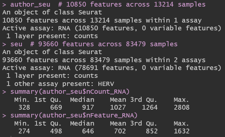
author_seu # 10850 features across 13214 samples
seu # 93660 features across 83479 samples
summary(author_seu$nCount_RNA)
summary(author_seu$nFeature_RNA)
# 改作者计数矩阵的细胞名
author_barcode <- sub("_.*$", "", colnames(author_counts))
author_individual <- sub("^[^_]+_", "", colnames(author_counts))
author_cell_id <- paste(author_barcode, author_individual, sep = "_")
colnames(author_counts) <- author_cell_id
# 改我的seu的细胞名
seu$individuals <- gsub("-", "_", seu$individuals)
rna_counts <- GetAssayData(seu, assay = "RNA", slot = "counts")
our_cell_names <- colnames(rna_counts)
our_barcode <- sub("^SRR[0-9]+_", "", our_cell_names)
our_barcode <- sub("-1$", "", our_barcode)
our_individuals <- seu$individuals[match(our_cell_names, rownames(seu@meta.data))]
our_cell_id <- paste(our_barcode, our_individuals, sep = "_")
seu$cell_id_qc <- our_cell_id
# 取交集
common_cells <- intersect(our_cell_id, colnames(author_counts))
our_idx <- match(common_cells, our_cell_id)
author_idx <- match(common_cells, colnames(author_counts))
our_sub <- rna_counts[, our_idx, drop = FALSE]
author_sub <- as.matrix(author_counts[, author_idx])
stopifnot(all(common_cells == colnames(author_sub)))
# 比较每个细胞的总UMI数
our_lib <- Matrix::colSums(our_sub)
author_lib <- Matrix::colSums(author_sub)
plot(
log10(author_lib + 1), log10(our_lib + 1),
xlab = "log10 UMI (author CSV)",
ylab = "log10 UMI (STARsolo)",
pch = 16, cex = 0.5,
)
abline(0, 1, col = "red")
cor(log10(author_lib + 1), log10(our_lib + 1), method = "pearson")
发现其实作者的计数矩阵是经过质控的,并且即使经过质控,UMI和基因数也不是很多
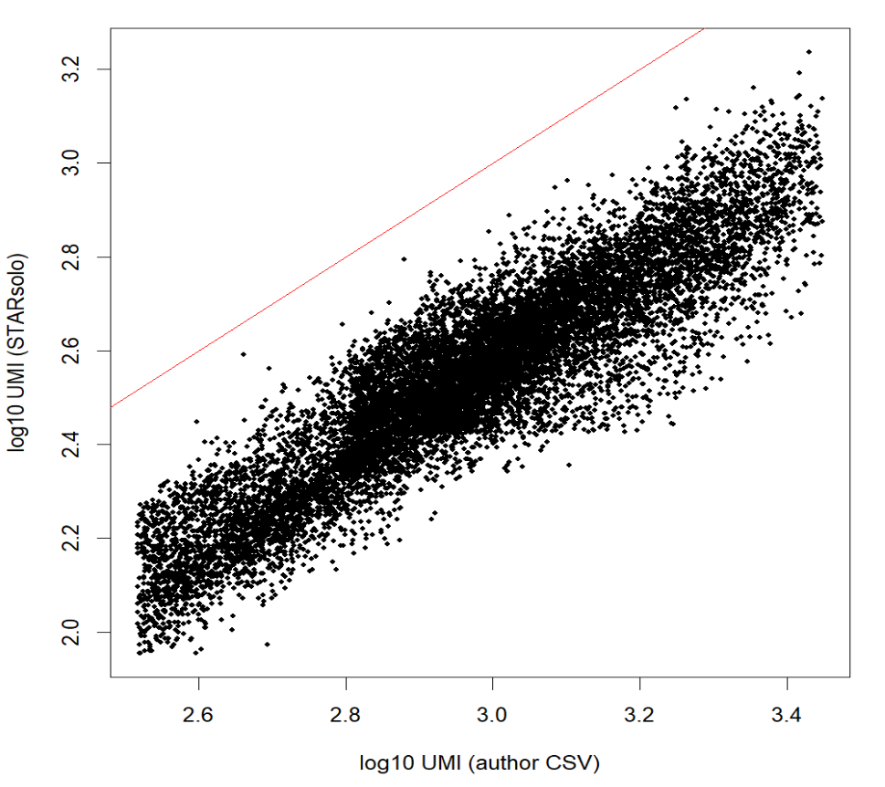
相关性>0.9,几乎是线性关系——我的计数和作者的高度相关,整体位于对角线以下可能是因为star比对的参数不同,比如feature模式、对多重比对或重复的处理策略、过滤低质量细胞等
看看hERV的具体情况:
DefaultAssay(seu) <- "HERV"
# 取表达最多的20个HERV
herv_sums <- Matrix::rowSums(herv_counts)
top_herv <- names(sort(herv_sums, decreasing = TRUE))[1:20]
VlnPlot(seu, features = head(top_herv, 6), group.by = "diagnosis", ncol = 3)  # 没有在所有样本中都特别高或者都为0的情况即可
# RNA和HERV总量的相关性
plot(
  log10(seu$nCount_RNA + 1),
  log10(seu$nCount_HERV + 1),
  pch = 16, cex = 0.3,
  xlab = "log10 nCount_RNA", ylab = "log10 nCount_HERV"
)  # 大致呈现左下-右上对角线分布
cor(log10(seu$nCount_RNA + 1), log10(seu$nCount_HERV + 1))  # 应该是有一些相关性的,不会完全是0,我这里是0.6多,正常
# QC图
VlnPlot(seu, features = c("nFeature_HERV", "nCount_HERV", "HERV_fraction"), group.by = "QCgroup", ncol = 3)
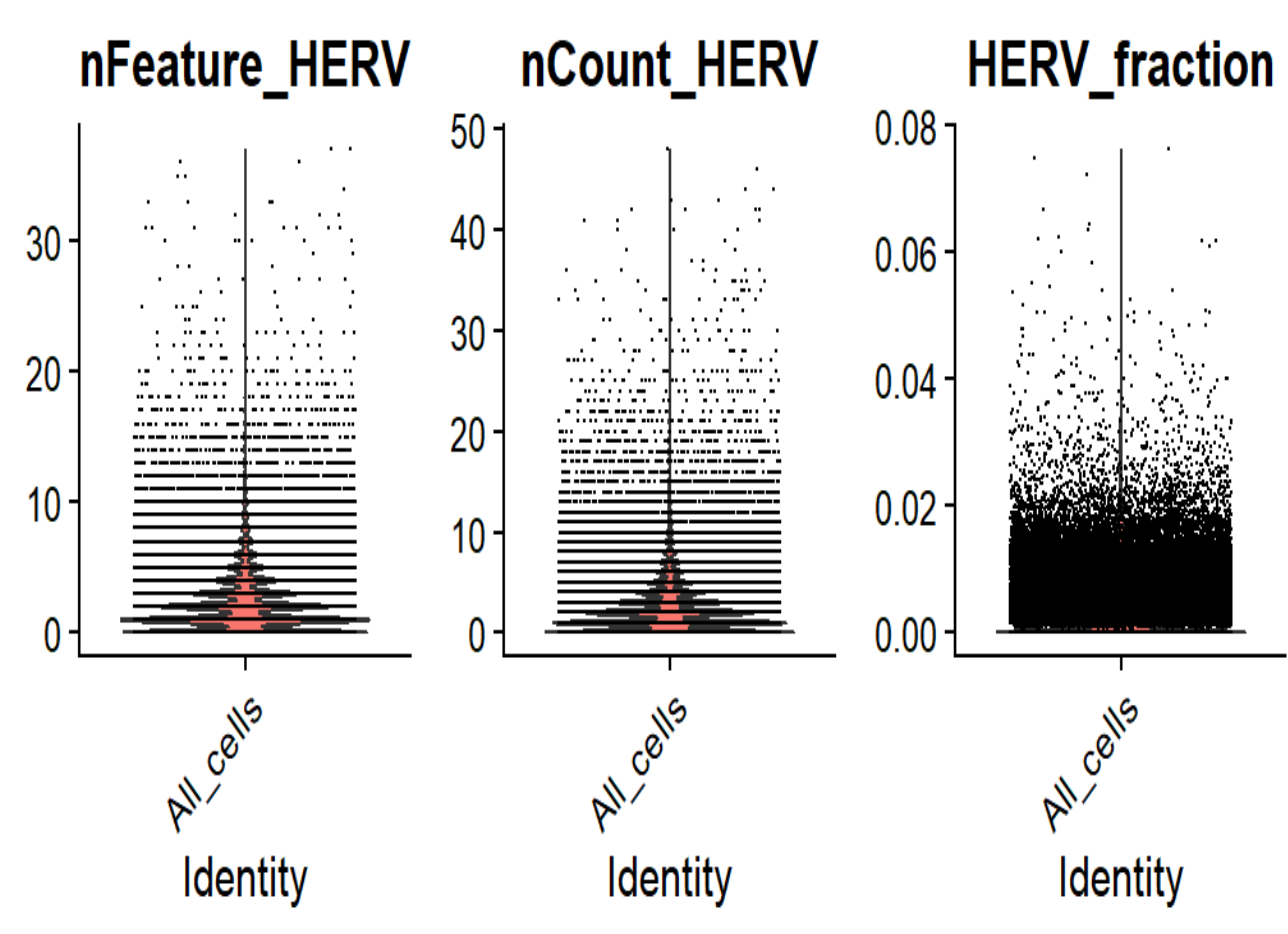
符合“不全为0、所有细胞hERV计数值不都很高”的情况
GSE157827
和上面GSE138852相比,同样都有作者提供的详细的计数矩阵+条形码+基因、都使用10X Genomics,但多了每个样本的注释信息(组别、性别、年龄、APOE等),同时数据量较大(共593.81G,碱基数2.02T,样本量21个)
点开其中一个样本的页面GSM4775561,可以看到是用什么测序技术测的(UMI和BC的位置和长度)
进入SRA run中下载
关键信息:
using the Chromium Single Cell 3′ Library Kit v3 (1000078; 10x Genomics)
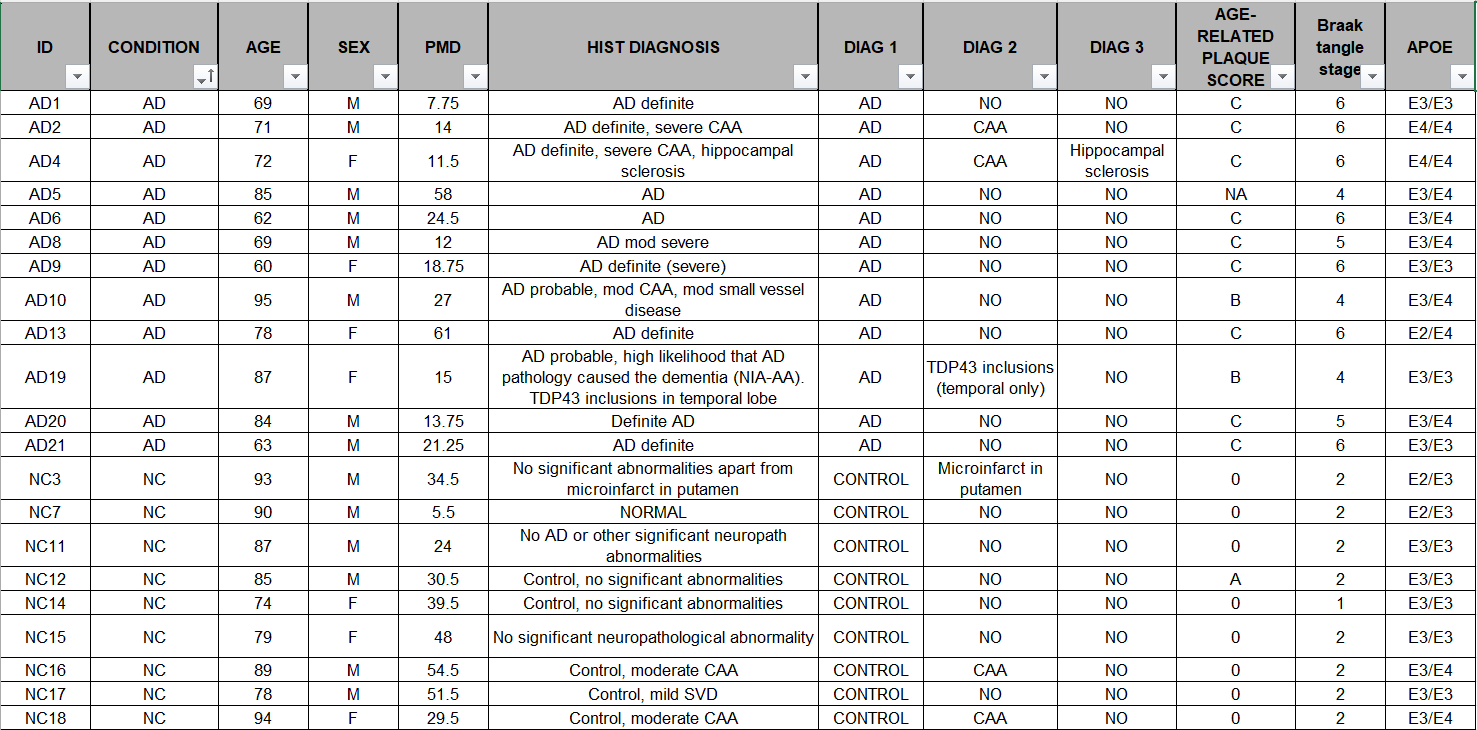
在相关论文Single-nucleus transcriptome analysis reveals dysregulation of angiogenic endothelial cells and neuroprotective glia in Alzheimer’s disease的补充材料Dataset_S01 (XLSX)中可以下载到每个样本的具体信息(组别、性别、年龄、APOE等):
同时还有一些国内的教程,例如复现2:AD与Normal细胞类型水平的差异基因挖掘,使用广泛
STAR比对
还是先看序列信息
zcat SRR12623876_1.fastq.gz | awk 'NR%4==2 {print length($0)}' | head
zcat SRR12623876_2.fastq.gz | awk 'NR%4==2 {print length($0)}' | head
-
SRRxxx_1.fastq.gz:26bp——UMI+barcode -
SRRxxx_2.fastq.gz:98bp——cDNA
whitelist:因为是v3版本,所以用3M-february-2018.txt
cd /public/home/wangtianhao/Desktop/GSE157827/
module load miniconda3/base
conda activate STAR
mkdir -p star/res
cd star
STAR \
  --runMode alignReads \
  --runThreadN 16 \
  --genomeDir /public/home/wangtianhao/Desktop/STAR_ref/hg38/ \
  --readFilesIn /public/home/wangtianhao/Desktop/GSE157827/fastq/SRR12623876_2.fastq.gz /public/home/wangtianhao/Desktop/GSE157827/fastq/SRR12623876_1.fastq.gz \
  --readFilesCommand zcat \
  --outFileNamePrefix res/SRR12623876_ \
  --soloType CB_UMI_Simple \
  --soloCBstart 1 \
  --soloCBlen 16 \
  --soloUMIstart 17 \
  --soloUMIlen 10 \
  --soloBarcodeReadLength 0 \
  --soloCBwhitelist /public/home/wangtianhao/Desktop/STAR_ref/whitelist/3M-february-2018.txt \
  --clipAdapterType CellRanger4 \
  --soloCBmatchWLtype 1MM_multi_Nbase_pseudocounts \
  --soloUMIfiltering MultiGeneUMI_CR \
  --soloUMIdedup 1MM_CR \
  --outSAMtype BAM SortedByCoordinate \
  --outSAMattributes NH HI nM AS CR UR CB UB GX GN sS sQ sM \
  --outSAMunmapped Within \
  --outFilterScoreMin 30 \
  --limitOutSJcollapsed 5000000 \
  --outFilterMultimapNmax 500 \
  --outFilterMultimapScoreRange 5
stellarscope计数
module load miniconda3/base
conda activate stellarscope
cd /public/home/wangtianhao/Desktop/GSE157827/
mkdir -p stellarscope/res
cd stellarscope
samtools view -@1 -u -F 4 -D CB:<(tail -n+1 /public/home/wangtianhao/Desktop/GSE157827/star/res/SRR12623876_Solo.out/Gene/filtered/barcodes.tsv) /public/home/wangtianhao/Desktop/GSE157827/star/res/SRR12623876_Aligned.sortedByCoord.out.bam | samtools sort -@16 -n -t CB -T ./tmp > ./res/Aligned.sortedByCB.bam
stellarscope assign \
  --exp_tag SRR12623876 \
  --outdir ./res \
  --nproc 16 \
  --stranded_mode F \
  --whitelist /public/home/wangtianhao/Desktop/GSE157827/star/res/SRR12623876_Solo.out/Gene/filtered/barcodes.tsv \
  --pooling_mode individual \
  --reassign_mode best_exclude \
  --max_iter 500 \
  --updated_sam \
  ./res/Aligned.sortedByCB.bam \
  /public/home/wangtianhao/Desktop/STAR_ref/transcripts.gtf
循环运行
workDir=/public/home/GENE_proc/wth/GSE157827/
genomeDir=/public/home/wangtianhao/Desktop/STAR_ref/hg38/
whitelist=/public/home/wangtianhao/Desktop/STAR_ref/whitelist/3M-february-2018.txt
hERV_gtf=/public/home/wangtianhao/Desktop/STAR_ref/transcripts.gtf
res_barcodes=barcodes
res_features=features
res_counts=counts
# STARsolo + stellarscope
cd ${workDir}
module load miniconda3/base
for SRR in $(cat ./fastq/SRR_Acc_List.txt); do
  conda activate STAR
  mkdir -p star
  STAR \
    --runMode alignReads \
    --runThreadN 16 \
    --genomeDir ${genomeDir} \
    --readFilesIn ./fastq/${SRR}_2.fastq.gz ./fastq/${SRR}_1.fastq.gz \
    --readFilesCommand zcat \
    --outFileNamePrefix star/${SRR}_ \
    --soloType CB_UMI_Simple \
    --soloCBstart 1 \
    --soloCBlen 16 \
    --soloUMIstart 17 \
    --soloUMIlen 10 \
    --soloBarcodeReadLength 0 \
    --soloCBwhitelist ${whitelist} \
    --clipAdapterType CellRanger4 \
    --soloCBmatchWLtype 1MM_multi_Nbase_pseudocounts \
    --soloUMIfiltering MultiGeneUMI_CR \
    --soloUMIdedup 1MM_CR \
    --outSAMtype BAM SortedByCoordinate \
    --outSAMattributes NH HI nM AS CR UR CB UB GX GN sS sQ sM \
    --outSAMunmapped Within \
    --outFilterScoreMin 30 \
    --limitOutSJcollapsed 5000000 \
    --outFilterMultimapNmax 500 \
    --outFilterMultimapScoreRange 5
  conda deactivate
  conda activate stellarscope
  mkdir -p stellarscope/${SRR}
  samtools view -@1 -u -F 4 -D CB:<(tail -n+1 ./star/${SRR}_Solo.out/Gene/filtered/barcodes.tsv) ./star/${SRR}_Aligned.sortedByCoord.out.bam | samtools sort -@16 -n -t CB -T ./tmp > ./stellarscope/${SRR}/Aligned.sortedByCB.bam
  stellarscope assign \
    --outdir ./stellarscope/${SRR} \
    --nproc 16 \
    --stranded_mode F \
    --whitelist ./star/${SRR}_Solo.out/Gene/filtered/barcodes.tsv \
    --pooling_mode individual \
    --reassign_mode best_exclude \
    --max_iter 500 \
    --updated_sam \
    ./stellarscope/${SRR}/Aligned.sortedByCB.bam \
    ${hERV_gtf}
  conda deactivate
done
# 汇总结果
cd ${workDir}
for SRR in $(cat ./fastq/SRR_Acc_List.txt); do
  mkdir -p mtx/${SRR}/gene
  cp ./star/${SRR}_Solo.out/Gene/filtered/barcodes.tsv ./mtx/${SRR}/gene/${res_barcodes}.tsv
  cp ./star/${SRR}_Solo.out/Gene/filtered/features.tsv ./mtx/${SRR}/gene/${res_features}.tsv
  cp ./star/${SRR}_Solo.out/Gene/filtered/matrix.mtx ./mtx/${SRR}/gene/${res_counts}.mtx
  mkdir -p mtx/${SRR}/hERV
  cp ./stellarscope/${SRR}/stellarscope-barcodes.tsv ./mtx/${SRR}/hERV/${res_barcodes}.tsv
  cp ./stellarscope/${SRR}/stellarscope-features.tsv ./mtx/${SRR}/hERV/${res_features}.tsv
  cp ./stellarscope/${SRR}/stellarscope-TE_counts.mtx ./mtx/${SRR}/hERV/${res_counts}.mtx
done
du -sh ./mtx  # 看看最后的数据有多大--400多M
# tar -czvf mtx.tar.gz ./mtx/
GSE233208
GEO界面,下载GSE233208_AD-DS_Cases.csv.gz样本信息
点开其中一个样本的页面GSM7412790,可以看到是用什么测序技术测的,关键信息:
using Parse biosciences Evercode WT kit (v1)
进入SRA run中,左面Assay Type选择RNA-Seq,下载41条数据(共732.66G,碱基数2.29T,样本数96个)
STAR比对
try 1
由于没找到官方提供的barcode whitelist,只能自己计算一下:统计推测的三段barcode中每种序列出现的频数,根据官方说法,可能有24/48/96个序列作为whitelist,观察生成的bc1_counts.txt,在96的地方有明显梯度,于是认为前96个序列位barcode
# 统计 BC1(11-18 位)的 8-mer 频数
zcat /public/home/wangtianhao/Desktop/GSE233208/1204test/fastq/SRR24710598_2.fastq.gz \
  | awk 'NR%4==2 {print substr($1,11,8)}' \
  | sort | uniq -c | sort -nr > /public/home/wangtianhao/Desktop/GSE233208/1204test/barcode/bc1_counts.txt
# 统计 BC2(49-56 位)
zcat /public/home/wangtianhao/Desktop/GSE233208/1204test/fastq/SRR24710598_2.fastq.gz \
  | awk 'NR%4==2 {print substr($1,49,8)}' \
  | sort | uniq -c | sort -nr > /public/home/wangtianhao/Desktop/GSE233208/1204test/barcode/bc2_counts.txt
# 统计 BC3(79-86 位)
zcat /public/home/wangtianhao/Desktop/GSE233208/1204test/fastq/SRR24710598_2.fastq.gz \
  | awk 'NR%4==2 {print substr($1,79,8)}' \
  | sort | uniq -c | sort -nr > /public/home/wangtianhao/Desktop/GSE233208/1204test/barcode/bc3_counts.txt
# 观察看出前96位的频数明显大于后面,因此截取前96位作为whitelist
# 过滤掉喊连续≥6碱基的条形码
cd /public/home/wangtianhao/Desktop/GSE233208/1204test/barcode/
grep -v -E 'A{6,}|C{6,}|G{6,}|T{6,}' bc1_counts.txt \
  | sort -k1,1nr \
  | head -96 \
  | awk '{print $2}' > bc1_whitelist.txt
grep -v -E 'A{6,}|C{6,}|G{6,}|T{6,}' bc2_counts.txt \
  | sort -k1,1nr \
  | head -96 \
  | awk '{print $2}' > bc2_whitelist.txt

# 因为第三段BC阶梯不明显,就扩大了一下范围
grep -v -E 'A{6,}|C{6,}|G{6,}|T{6,}' bc3_counts.txt \
  | sort -k1,1nr \
  | head -200 \
  | awk '{print $2}' > bc3_whitelist.txt
一定一定注意--readFilesIn参数的设置,第一个fastq是cDNA,第二个是UMI和barcode
- 本来不想设置
--soloCBwhitelist过滤的,但STAR官方好像强制要求这个参数,只能用上面的方法生成一个不太严谨的whitelist——只有barcode出现在这个whitelist里的读段才算有效读段
cd /public/home/wangtianhao/Desktop/GSE233208/1204test/
module load miniconda3/base
conda activate STAR
mkdir -p starsolo
# 注意以下命令执行时删掉#的行,否则只读到第一个#就不往下读了
STAR \
  --runMode alignReads \
  --runThreadN 16 \
  --genomeDir /public/home/wangtianhao/Desktop/STAR_ref/hg38/ \
  --readFilesIn /public/home/wangtianhao/Desktop/GSE233208/1204test/fastq/SRR24710598_1.fastq.gz /public/home/wangtianhao/Desktop/GSE233208/1204test/fastq/SRR24710598_2.fastq.gz \
  --readFilesCommand zcat \
  --outFileNamePrefix starsolo/SRR24710598_ \
  # 单细胞模式
  --soloType CB_UMI_Complex \
  --soloCBwhitelist /public/home/wangtianhao/Desktop/GSE233208/1204test/barcode/bc1_whitelist.txt /public/home/wangtianhao/Desktop/GSE233208/1204test/barcode/bc2_whitelist.txt /public/home/wangtianhao/Desktop/GSE233208/1204test/barcode/bc3_whitelist.txt \
  --soloCBmatchWLtype 1MM \
  # 条形码
  --soloUMIposition 0_0_0_9 \
  --soloCBposition 0_10_0_17 0_48_0_55 0_78_0_85 \
  # 计数/细胞筛选设置
  --soloFeatures GeneFull \
  --soloCellFilter EmptyDrops_CR \
  --soloMultiMappers EM \
  # BAM输出和Tags(给Stellarscope用)
  --outSAMtype BAM SortedByCoordinate \
  --outSAMattributes NH HI nM AS CR UR CB UB GX GN sS sQ sM \
  # Stellarscope要求保留多重比对
  --outSAMunmapped Within \
  --outFilterMultimapNmax 500 \
  --outFilterMultimapScoreRange 5
结果虽然从条形码的角度对的上,但没有样本id也没什么用
try 2
找了一个野生工具Analysis tools for split-seq,作者使用自己创作的解码(条形码和sample组别)方式,没有依赖splitpipe,但更新时间是5年前,有一些古老
# 安装
git clone https://github.com/yjzhang/split-seq-pipelinec
# git clone https://ghfast.top/https://github.com/yjzhang/split-seq-pipeline
export PATH=$PATH:$HOME/split-seq-pipeline/

# 配置环境
module load miniconda3/base
conda create -n split-seq \
  python=3.8 \
  samtools=1.9 \
  numpy pysam pandas scipy matplotlib

# 因为他用的旧版本STAR,只能用源码编译的方式安装
cd ~
wget https://github.com/alexdobin/STAR/archive/2.6.1c.tar.gz
tar -xzf 2.6.1c.tar.gz
cd STAR-2.6.1c
cd source
make STAR
要求必须使用他的方式重建STAR索引,自己建的会缺一个他统计的pkl文件
# 建索引
module load miniconda3/base
conda activate split-seq
# 为了避免与其他版本STAR冲突,只在运行他这个pipeline的时候才把2.6.1的STAR加入环境变量
export PATH=$PATH:$HOME/STAR-2.6.1c/bin/Linux_x86_64/
split-seq mkref \
  --genome hg38 \
  --fasta /public/home/wangtianhao/Desktop/STAR_ref/GRCh38.p14.genome.fa \
  --genes /public/home/wangtianhao/Desktop/STAR_ref/gencode.v49.annotation.gtf \
  --output_dir /public/home/wangtianhao/Desktop/STAR_ref/hg38_split-seq/ \
  --nthreads 16
之后就可以开始比对,经过实测他示例中的参数--chemistry v2应该是适配这套数据的
module load miniconda3/base
conda activate split-seq
export PATH=$PATH:$HOME/STAR-2.6.1c/bin/Linux_x86_64/
mkdir -p /public/home/wangtianhao/Desktop/GSE233208/1205test/AD_S8_L004/
split-seq all \
  --fq1 /public/home/wangtianhao/Desktop/GSE233208/1205test/fastq/AD_S8_L004_R1.fastq.gz \
  --fq2 /public/home/wangtianhao/Desktop/GSE233208/1205test/fastq/AD_S8_L004_R2.fastq.gz \
  --output_dir /public/home/wangtianhao/Desktop/GSE233208/1205test/AD_S8_L004/ \
  --chemistry v2 \
  --genome_dir /public/home/wangtianhao/Desktop/STAR_ref/hg38_split-seq/ \
  --nthreads 16 \
  --sample '28' A1-A4 \
  --sample '16' A5-A8 \
  --sample '94' A9-A12 \
  --sample '88' B1-B4 \
  --sample '131' B5-B8 \
  --sample '19' B9-B12 \
  --sample '107' C1-C4 \
  --sample '101' C5-C8 \
  --sample '10' C9-C12 \
  --sample '63' D1-D2 \
  --sample '128' D3-D4 \
  --sample '50' D5-D6 \
  --sample '100' D7-D8 \
  --sample 'humAD-87' D9-D10 \
  --sample '20' D11-D12
在分析的末尾,作者的split_seq/analysis.py文件中的generate_single_dge_report报错KeyError(f"{not_found} not in index"),仔细一看是一段对Fraction Reads in Cells统计的代码出错,感觉这个数据不太重要,于是注释掉了该文件中所有类似统计的行(527-531、540-541、546、574、576-583)
结果:处理一条数据大约需要6-7个小时,确实可以得到看起来很正确的统计结果,包括每个样本id对应的计数矩阵+条形码+基因,作者筛选出来有有效条形码的读段fastq文件极其比对结果bam,理论上可以根据这个结果来构建Seurat对象
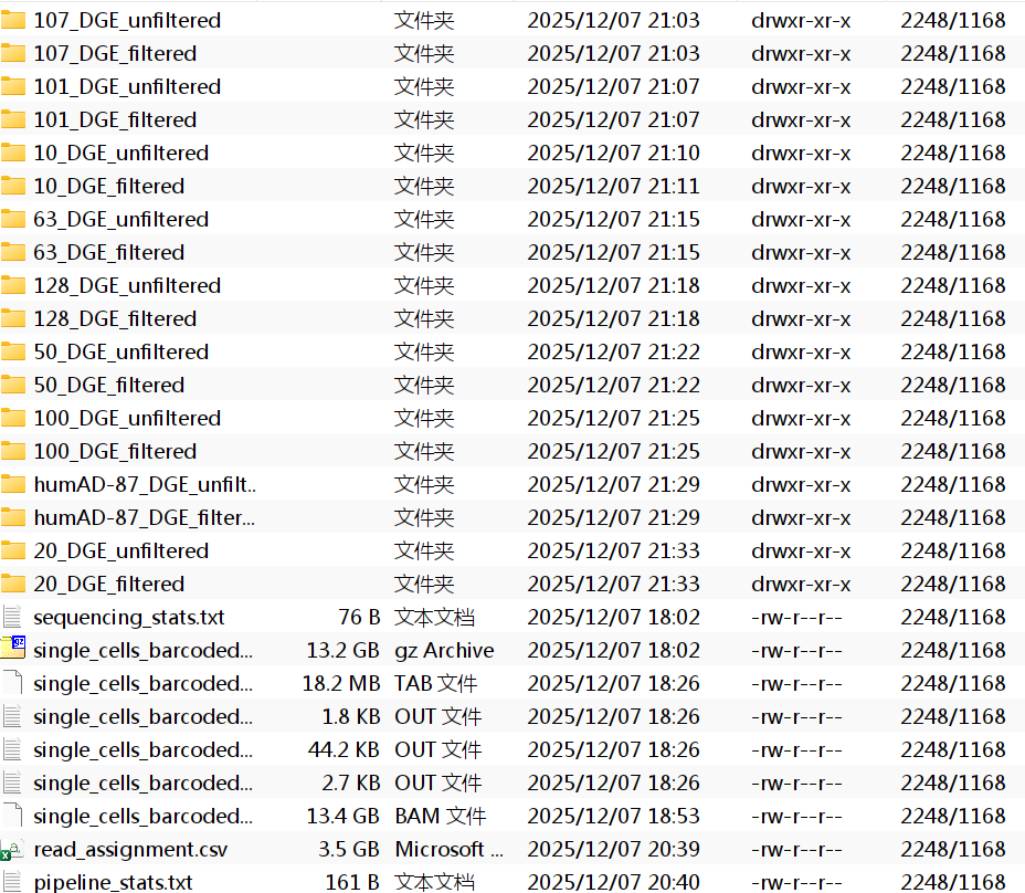
每个样本ID都对应一个文件夹,每个文件夹内有cell_metadata.csv/DGE.mtx/genes.csv三个文件
-
cell_metadata.csv: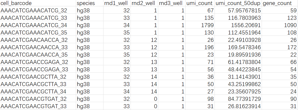
-
genes.csv: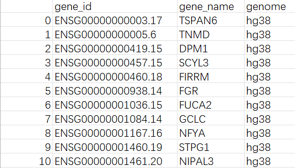
问题:
- 虽然有类似的结果,但不能确定这个GitHub项目处理的流程是否正确,毕竟是野生项目,有可能只是作者给自己使用的数据写的,无法推广到这个比较偏门的数据。最主要这个结果的正确性是无法验证的(除非跑完整个流程后再到Seurat里面画图查看)
- 需要与后续stellarscope分析衔接,因为作者使用自己写的流程,不知道是否保留了后面stellarscope需要的文件,而且尚未清楚是怎么筛选的、筛选结果的格式是什么,需要进一步根据stellarscope的输入和这个pipeline的输出进行研究
验证野生pipeline结果是否正确
大体思路:将作者提供的Seurat对象中对应批次(batch5_Sublibrary_8_S8_L004、batch5_Sublibrary_7_S7_L004)的细胞提取出来,再用我们测出来的两组数据构建Seurat对象,最后将这两个Seurat对象进行比较
收集计数矩阵:
cp -r /public/home/wangtianhao/Desktop/GSE233208/1205test/AD_S7_L004/*_DGE_filtered /public/home/wangtianhao/Desktop/GSE233208/1205test/mtx/AD_S7_L004/
cp -r /public/home/wangtianhao/Desktop/GSE233208/1205test/AD_S8_L004/*_DGE_filtered /public/home/wangtianhao/Desktop/GSE233208/1205test/mtx/AD_S8_L004/
du -sh /public/home/wangtianhao/Desktop/GSE233208/1205test/mtx/  # 2个sublibrary-2G
cd /public/home/wangtianhao/Desktop/GSE233208/1205test
tar -czvf mtx.tar.gz ./mtx/
将作者提供的Seurat对象中对应批次的提取出来:
sn <- readRDS("C:\\Users\\17185\\Desktop\\hERV_calc\\GSE233208\\data\\GSE233208_human_snRNA_subset.rds")
# sn <- readRDS("/public/home/wangtianhao/Desktop/GSE233208/raw_data/GSE233208_Human_snRNA-Seq_ADDS_integrated.rds")
meta <- sn@meta.data
cells_batch5_s7s8 <- meta %>%
  filter(
    Batch == "Batch5",
    Sublibrary %in% c("Sublibrary_7_S7", "Sublibrary_8_S8")
  ) %>%
  rownames()
sn_b5_s7s8 <- subset(sn, cells = cells_batch5_s7s8)
# 解决Seurat5.3版本的Error in validObject(object = object) : invalid class “DimReduc” object: dimension names for ‘cell.embeddings’ must be positive integers报错
# sn_b5_s7s8 <- DietSeurat(sn_b5_s7s8, dimreducs = character())
meta <- sn_b5_s7s8@meta.data
suffix <- case_when(
  str_detect(meta$Sublibrary, "S7$") ~ "7",
  str_detect(meta$Sublibrary, "S8$") ~ "8",
)
new_cellnames <- paste0(meta$cell_barcode, "_", suffix)
stopifnot(!any(duplicated(new_cellnames)))
rename_vec <- setNames(
  new_cellnames,
  colnames(sn_b5_s7s8)
)
sn_b5_s7s8 <- RenameCells(sn_b5_s7s8, new.names = rename_vec)
sn_b5_s7s8$cell_barcode_sub <- colnames(sn_b5_s7s8)
View(sn_b5_s7s8@meta.data)
saveRDS(
  sn_b5_s7s8,
  file = "C:\\Users\\17185\\Desktop\\hERV_calc\\GSE233208\\data\\GSE233208_Batch5_S7S8.rds",
  # file = "/public/home/wangtianhao/Desktop/GSE233208/data/GSE233208_Batch5_S7S8.rds",
  compress = "xz"
)
rm(list = ls())
sn_b5_s7s8 <- readRDS("C:\\Users\\17185\\Desktop\\hERV_calc\\GSE233208\\data\\GSE233208_Batch5_S7S8.rds")
最后剩下15449个细胞
> sn_b5_s7s8
An object of class Seurat
29889 features across 15449 samples within 1 assay
Active assay: RNA (29889 features, 0 variable features)
 2 layers present: counts, data
合并我使用野生pipeline得到的计数矩阵:
# 读取一个计数矩阵的函数
base_dir <- "C:\\Users\\17185\\Desktop\\hERV_calc\\GSE233208\\data\\split-seq_res"
sublibs <- c("AD_S7_L004", "AD_S8_L004")
sub_suffix <- c("AD_S7_L004" = "_7", "AD_S8_L004" = "_8")
seu_list <- list()
read_one_sample <- function(sd, suffix, sample_id) {
  features <- read.csv(file.path(sd, "genes.csv")) %>%
    select(gene_id, gene_name) %>%
    write_tsv(file = file.path(sd, "genes.tsv"), col_names = F)
  barcode <- read.csv(file.path(sd, "cell_metadata.csv")) %>%
    select(cell_barcode) %>%
    write_tsv(file = file.path(sd, "barcodes.tsv"), col_names = F)
  m <- readMM(file.path(sd, "DGE.mtx"))
  writeMM(t(m), file.path(sd, "DGE_T.mtx"))
  gene_counts <- ReadMtx(
    mtx = file.path(sd, "DGE_T.mtx"),
    features = file.path(sd, "genes.tsv"),
    cells = file.path(sd, "barcodes.tsv")
  )
  colnames(gene_counts) <- paste0(colnames(gene_counts), suffix)
  seu <- CreateSeuratObject(
    counts = gene_counts,
    assay = "RNA",
    project = "ADDS_2021"
  )
  seu$sample_id <- sample_id
  return(seu)
}
# 循环读取所有矩阵
for (sdir in sublibs) {
  sublib_path <- file.path(base_dir, sdir)
  sample_dirs <- list.dirs(sublib_path, full.names = TRUE, recursive = FALSE)
  sample_dirs <- sample_dirs[grepl("DGE_filtered$", basename(sample_dirs))]
  suffix <- sub_suffix[[sdir]]
  for (sd in sample_dirs) {
    sample_name <- basename(sd)
    sample_id <- sub("_DGE_filtered$", "", sample_name)
    seu <- read_one_sample(sd, suffix, sample_id)
    seu_list[[paste(sdir, sd, sep = '_')]] <- seu
  }
}
sn_my <- Reduce(function(x, y) merge(x, y), seu_list)
rm(seu_list)
# 合并每个layers
sn_my <- JoinLayers(sn_my, assay = "RNA")
# 添加metadata,并使这两个Seurat对象结构一致
sample_meta <- read.csv("C:\\Users\\17185\\Desktop\\hERV_calc\\GSE233208\\GSE233208_AD-DS_Cases.csv")
select_cols <- c("nCount_RNA", "nFeature_RNA", "SampleID", "Age", "Sex", "PMI", "APoE", "DX", "cell_barcode_sub")
meta_df <- sn_my@meta.data %>%
  mutate(
    SampleID = sample_id,
    cell_barcode_sub = rownames(sn_my@meta.data)
  ) %>%
  left_join(sample_meta, by = "SampleID") %>%
  select(select_cols)
rownames(meta_df) <- meta_df$cell_barcode_sub
sn_my@meta.data <- meta_df
sn_b5_s7s8@meta.data <- sn_b5_s7s8@meta.data %>%
  select(select_cols)
View(sn_b5_s7s8@meta.data)
View(sn_my@meta.data)
saveRDS(
  sn_my,
  file = "C:\\Users\\17185\\Desktop\\hERV_calc\\GSE233208\\data\\my_Batch5_S7S8.rds",
  compress = "xz"
)
sn_my <- readRDS("C:\\Users\\17185\\Desktop\\hERV_calc\\GSE233208\\data\\my_Batch5_S7S8.rds")
# 看看细胞名是否添加成功
my_rna_counts <- GetAssayData(sn_my, assay = "RNA", slot = "counts")
View(my_rna_counts)  # 有没有dimNames
rna_counts <- GetAssayData(sn_b5_s7s8, assay = "RNA", slot = "counts")
View(rna_counts)  # 结构是否差不多
剩下的细胞和基因数量都比作者的多:(后面一起分析原因)
> sn_my
An object of class Seurat
50319 features across 728585 samples within 1 assay
Active assay: RNA (50319 features, 0 variable features)
 1 layer present: counts
有一个奇怪的问题:其实在最早GSE138852建Seurat对象时就有,但我到这才发现
如图,在View(my_sn)的界面,橙色框里面的Dimnames为null,但实际上如果我my_rna_counts <- GetAssayData(sn_my, assay = "RNA", slot = "counts")后,在View(my_rna_counts)的界面,同样的位置又可以正常显示细胞名和基因名
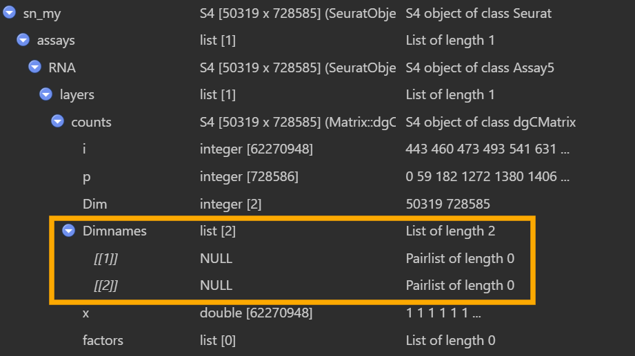
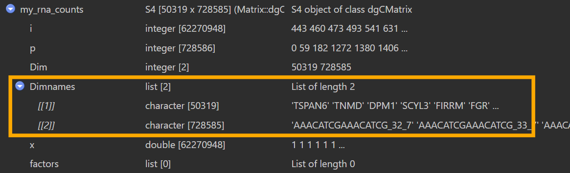
据说是正常现象,是Seurat v5的特性,RNA是一个Assay5对象,表达矩阵存在layers里,而“基因名/细胞名”由Assay5在assay层面单独管理,通过dimnames(Assay5)方法获取/设置。上面在第一个View里面看到的是sn_my[["RNA"]]@layers$counts这个dgCMatrix本体,不包含dimnames,而GetAssayData时会按assay保存的基因名/细胞名把dimnames补回去,所以后面就能看到了。因此在后面分析时,要使用Seurat的正规接口,不要自己去操作底层对象
验证结果:首先验证样本id-barcode是否对应
cells_my <- colnames(sn_my)
cells_auth <- colnames(sn_b5_s7s8)
length(cells_my)  # 728585
length(cells_auth)  # 15449
common_cells <- intersect(cells_my, cells_auth)
length(common_cells)  # 15449
all(cells_auth %in% cells_my)  # TRUE
length(rownames(my_rna_counts))  # 50319
length(rownames(rna_counts))  # 29889
common_genes <- intersect(
  rownames(my_rna_counts),
  rownames(rna_counts)
)
length(common_genes)  # 19159
这里发现作者的细胞全在我的细胞中,可能是作者设置了筛选,而我的是原始结果(pipeline直接用普通STAR比对,在STAR时就没有筛选,后续也没有设置筛选的命令),然后作者的基因数也比较少(我的是5w,作者的是3w),最后取交集后剩2w(可能是作者的基因集版本和我的不同,我的gtf注释版本、基因范围可能更宽,或者作者过滤掉了低表达基因)。因此将两个计数矩阵取交集,只保留作者的基因/细胞
# 矩阵取交集
my_mat <- my_rna_counts[common_genes, common_cells, drop = FALSE]
auth_mat <- rna_counts[common_genes, common_cells, drop = FALSE]
# Seurat对象取交集(因为后面Seurat对象只比较细胞名,就只取了细胞名的交集)
sn_my_common <- subset(
  sn_my,
  subset = cell_barcode_sub %in% common_cells
)
继续验证样本id-barcode是否对应
# 各自的SampleID分布
table(sn_my_common$SampleID)
table(sn_b5_s7s8$SampleID)  # SampleID是相同的
sample_ids <- intersect(
  unique(sn_my_common$SampleID),
  unique(sn_b5_s7s8$SampleID)
)
sample_check <- lapply(sample_ids, function(sid) {
  cells_my_sid <- colnames(sn_my_common)[sn_my_common$SampleID == sid]
  cells_auth_sid <- colnames(sn_b5_s7s8)[sn_b5_s7s8$SampleID == sid]
  list(
    SampleID = sid,
    n_my = length(cells_my_sid),  # 某个样本中我的细胞数
    n_auth = length(cells_auth_sid),  # 作者的细胞数
    n_overlap = length(intersect(cells_my_sid, cells_auth_sid)),  # 重叠的细胞数
    my_not_auth = length(setdiff(cells_my_sid, cells_auth_sid)),
    auth_not_my = length(setdiff(cells_auth_sid, cells_my_sid))  # 哪一边多出来的细胞(如果都是0就是完全一致)
  )
})
View(do.call(rbind, lapply(sample_check, as.data.frame)))
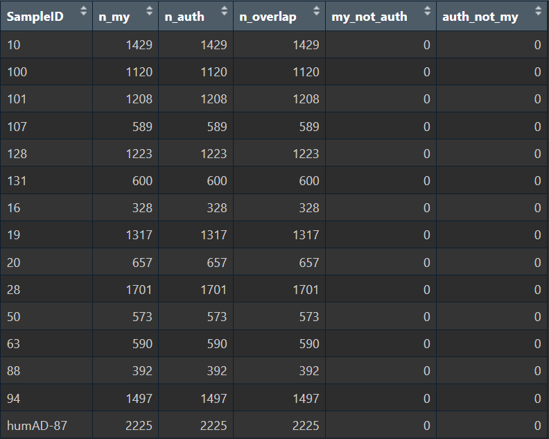
在以上步骤中,我先把我的Seurat对象根据作者Seurat对象的barcode进行提取,这样就起到一个过滤的作用;之后按样本ID分组,比较每个样本ID内,我的barcode和作者的是否相同。可以看到两组样本ID-barcode的对应关系完全相同,说明野生pipeline的样本id和barcode提取方式是正确的
比较两个计数矩阵的差异
QC:每个cell/每个gene的总UMI&检出基因数
# 每个细胞的总UMI
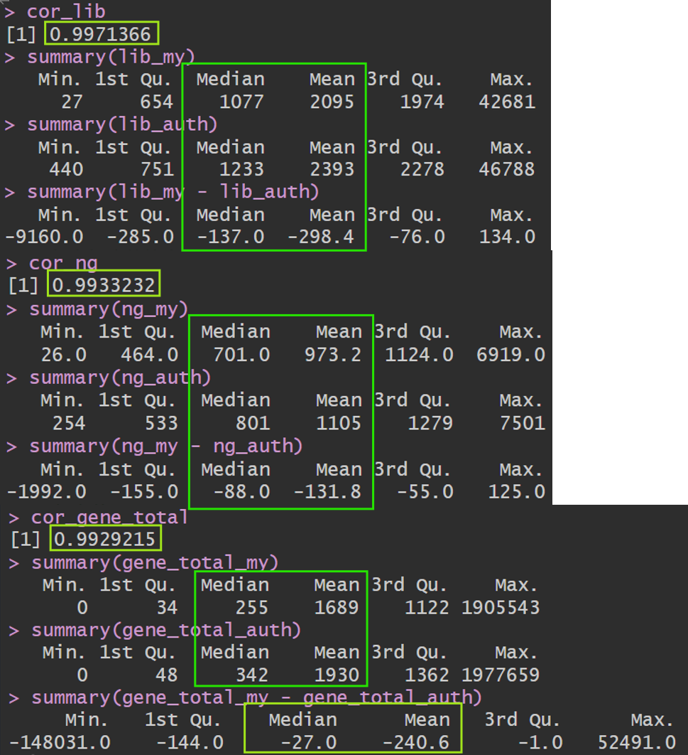
lib_my <- Matrix::colSums(my_mat)
lib_auth <- Matrix::colSums(auth_mat)
cor_lib <- cor(lib_my, lib_auth)
cor_lib
summary(lib_my)
summary(lib_auth)
summary(lib_my - lib_auth)
# 每个细胞的检出基因数(count>0)
ng_my <- Matrix::colSums(my_mat > 0)
ng_auth <- Matrix::colSums(auth_mat > 0)
cor_ng <- cor(ng_my, ng_auth)
cor_ng
summary(ng_my)
summary(ng_auth)
summary(ng_my - ng_auth)
# 每个基因
gene_total_my <- Matrix::rowSums(my_mat)
gene_total_auth <- Matrix::rowSums(auth_mat)
cor_gene_total <- cor(gene_total_my, gene_total_auth)
cor_gene_total
summary(gene_total_my)
summary(gene_total_auth)
summary(gene_total_my - gene_total_auth)
几乎是贴着对角线分布,低表达区域有一些散点在对角线附近发散,这是由于1->2、0->1这种对(ln(x+1))来说差别比较大,但实际差别不大,属于正常现象
v_my <- as.vector(log1p(my_mat))
v_auth <- as.vector(log1p(auth_mat))
cor_flat <- cor(v_my, v_auth)
cor_flat  # 0.927427
# 抽取3k个细胞×3k个基因画个散点图
cells_sample <- sample(colnames(my_mat), 3000)
genes_sample <- sample(rownames(my_mat), 3000)
my_sub <- as.matrix(my_mat[genes_sample, cells_sample])
auth_sub <- as.matrix(auth_mat[genes_sample, cells_sample])
v_my_sub <- as.vector(log1p(my_sub))
v_auth_sub <- as.vector(log1p(auth_sub))
par(pin = c(10, 10))
plot(v_my_sub, v_auth_sub, pch = ".", xlab = "log1p(my)", ylab = "log1p(author)")
abline(0, 1, col = "red")
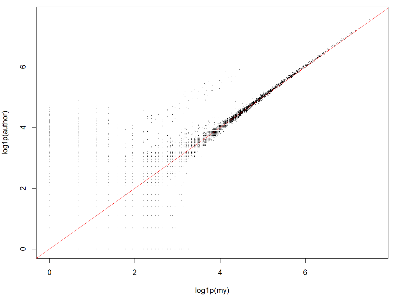
总体来看我的计数和作者的计数相似度还是蛮高的,虽然总体UMI略微偏低而基因数偏高(大概率是因为计数策略差异,作者更宽松的保留了多重比对,以及前面说过的使用的gtf注释不同)
# 差异是否均匀分布在所有sample上
lib_diff_df <- data.frame(
  cell = common_cells,
  lib_my = lib_my,
  lib_auth = lib_auth,
  diff = lib_my - lib_auth
)
lib_diff_df$SampleID <- sn_b5_s7s8$SampleID[match(lib_diff_df$cell, colnames(sn_b5_s7s8))]
View(lib_diff_df %>%
  group_by(SampleID) %>%
  summarise(
    mean_diff = mean(diff),
    median_diff = median(diff)
  ))
# 看看有没有某些基因在两个pipeline之间差异特别大
eps <- 1
log_my <- log2(gene_total_my   + eps)
log_auth <- log2(gene_total_auth + eps)
A <- (log_my + log_auth) / 2
M <- log_my - log_auth
ma_df <- data.frame(
  gene = rownames(my_mat),
  A = A,
  M = M
)
keep <- (gene_total_my + gene_total_auth) >= 10
ma_df_filt <- ma_df[keep, ]
ggplot(ma_df_filt, aes(x = A, y = M)) +
  geom_point(alpha = 0.3, size = 0.4) +
  geom_hline(yintercept = 0, colour = "red") +
  labs(
    x = "A = mean log2(count)",
    y = "M = log2(my) - log2(author)",
    title = "Gene-level MA plot: my pipeline vs author"
  ) +
  theme_bw()
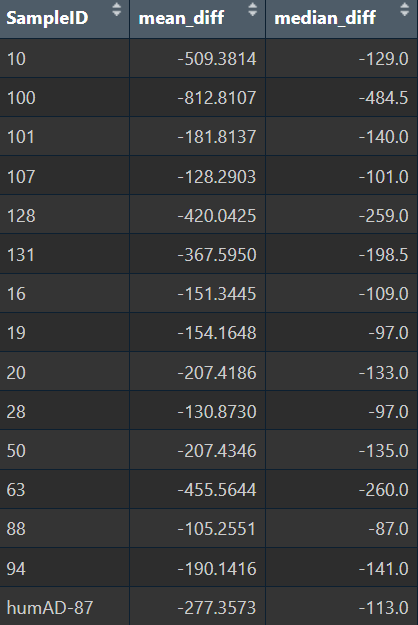
- 所有样本的diff都是负值,方向一致;差异的数量级也相同,有一点波动但不多,说明不是某几个样本导致总体的差异
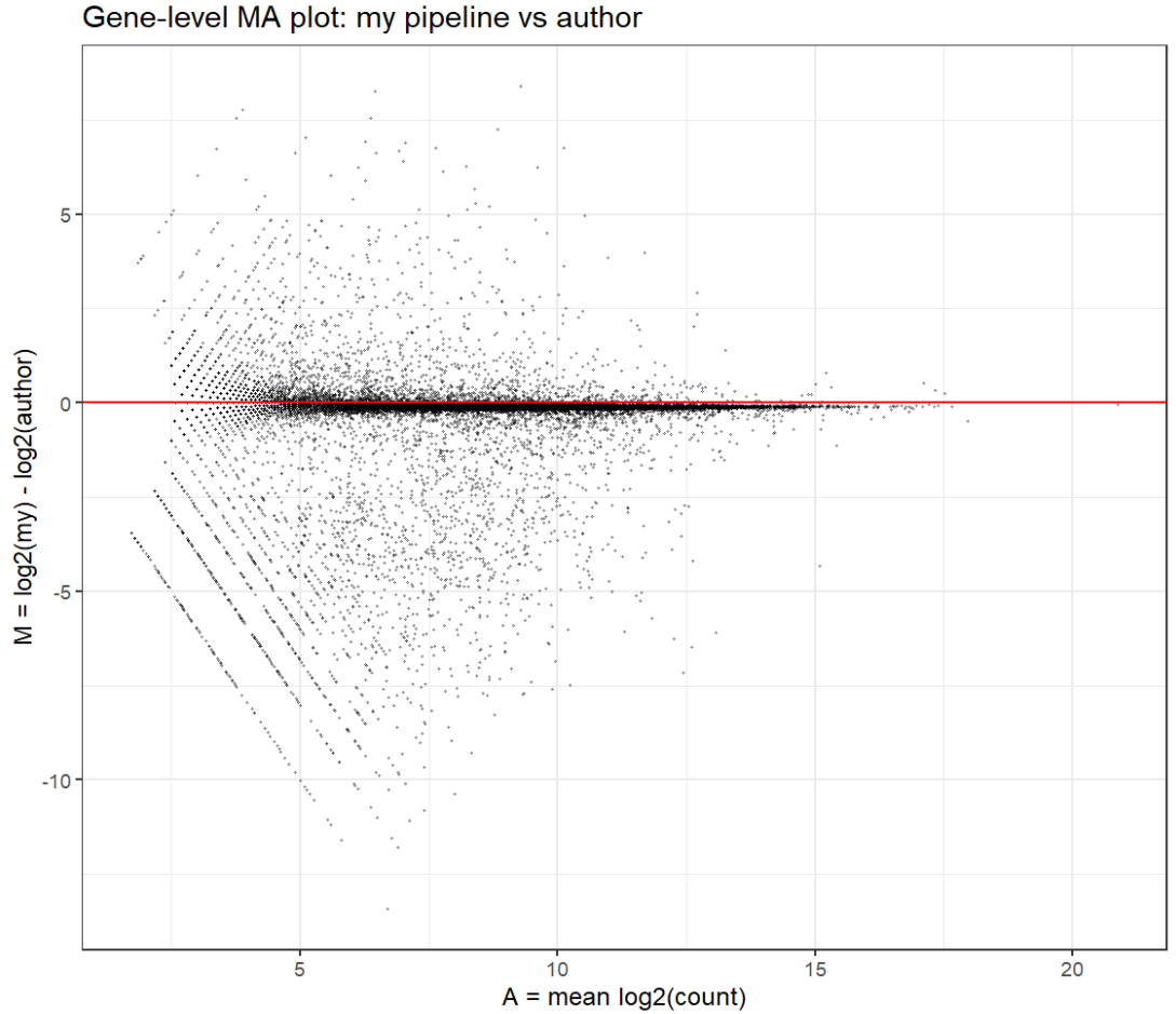
- 中高表达基因与作者的结果一致性比较高(围绕0对称、离散度适中),低表达基因计数更少(更容易把低计数变成0,或者更少地分配多重比对),是一种“低计数事件更保守”的模式,而不是因为某些特定基因而导致总体差异
总结:野生pipeline的“识别barcode”以及“根据sampleID分组”的功能是没有问题的,在计数上识别的基因数偏高而UMI偏低,但总体相似度很高,问题不大。最主要的是需要加一个细胞过滤的功能,并且野生pipeline识别基因的方式可能与作者略有不同,后续需要注意(比如也加一个低表达基因过滤之类的)
一些小讨论
普通基因和hERV计数矩阵的标准化方法
-
分别标准化:对于RNA assay用“该细胞的基因总UMI”当分母,对HERV assay用“该细胞的hERV总UMI”当分母,最后得到的结果是“RNA assay-这个基因在该细胞中的相对丰度(相对于细胞内所有基因的总UMI)”+“HERV assay这个hERV位点在该细胞中的相对丰度(相对于细胞内所有hERV UMI)”
如果只是探究“某个基因在不同细胞/分组中的差异”和“某个hERV在不同细胞/分组中的差异”,就可以分别标准化,不会影响“横向比较不同细胞”的结论
但如果想要把基因和hERV放在一起比较/探究相关性,比如看“某个hERV位点的表达和某个AD风险基因的表达有没有相关”,或者建一个
Gene ~ hERV + xxx的模型,或者探究“某个细胞hERV表达高,同时哪些基因被上调”……这类跨assay的研究,正则化出来的数值可能会被“不同分母”强烈影响,导致可解释性差一个极端点的例子,有三个细胞A、B、C,都表达了G基因,UMI分别是10、20、30,也都表达了H的hERV位点,UMI分别是2、4、6,这时G和H就是完全正相关的情况,如果分别标准化,对于基因来说,由于一个细胞会表达很多基因,所以标准化后可能还是0.01/0.02/0.03,但hERV在每个细胞内表达量很少,很有可能一个细胞只有几个hERV位点计数很高,假设这三个细胞只表达了H,那么标准化后就是1/1/1,相关性消失,而放在一起标准化后,就是2/12、4/24、6/36,仍有相关性
-
放在一起标准化:用同一套size factor(库深度因子)同时标准化基因和hERV,最后RNA和HERV的log标准化值用的是同一套总UMI作分母
- 把基因+hERV合成一个大矩阵再标准化一次
- 用RNA的库深度去标准化hERV:即用基因counts定义每个细胞的size factor,再自己手动用这套size factor去标准化hERV,对RNA assay仍然用正常的
NormalizeData(seu, assay = "RNA")
标准化函数会通过log操作把hERV和基因的UMI压到同一数量级,所以不用担心hERV的UMI过小而影响后续分析,而且回归分析这类的结果实际上是不受“很小的数”的影响的
再具体一点来说,用RNA assay做QC、PCA、UMAP、聚类、细胞类型注释,对HERV assay用和RNA同一个库深度因子来做标准化,然后再在同一细胞类型内做AD-Control的HERV差异表达、HERV-AD风险基因表达相关性、HERV_fraction等指标与细胞状态、病理特征的关联分析
为什么更推荐“用RNA的库深度去标准化hERV”:易操作——这样不用动RNA assay,RNA assay还是用正常的分析方法,只是在此基础上加一个hERV的视角;不让hERV影响库深度的定义——如果用第一种,在少部分HERV特别高的细胞里,库深度会突然被放大,而这部分变化其实是你感兴趣的signal本身,一边拿来做分母,一边还想研究它,就容易把signal抹掉一部分(基因数多、信号平滑,适合估计测序深度;而hERV稀疏而极端,更适合当“响应变量”,不适合当“校正因子”)
- 如果想研究“所有转录本的全集”(基因+HERV+其它TE),想从最原始的读段数出发,做一个完全统一的大模型,就可以用第一种方法
- 通常要做的分析都是在“RNA定义的细胞世界”里加一个HERV视角,而不是让hERV反过来定义世界观,因此大多数类似研究都是用基因计数作为size factor
- 数学上两种方法的size factor差异不大,实践上更偏向第二种方法
总结一下,统一标准化的根本原因,不是“因为这是两个不同assay”,而是“我们要分析这两个assay的相关性,即cor(gene, hERV)和gene ~ hERV + covariates,要求这些数值的相对量纲必须可比”,同时hERV的计数结构很极端(总量少,少数hERV位点占主导),放大了这种矛盾(hERV单独标准化后各细胞都差不多,无法与基因检测相关性),因此说统一标准化是需要的
AI Agent
AI Agent:简单来说就是“会自己想下一步干啥、会自己调用工具、会自己循环迭代”的AI,不同于GPT这样问一句答一句的,它更像一个能跑流程的智能脚本——在大模型之上,加了一层“循环+规划+调用工具”的逻辑,让它像一个半自动脚本工程师一样完成一个完整流程。具体来说,有大致以下几个特点
- 有目标(Goal):接受一个比较大的任务,例如“帮我从原始fastq到Seurat对象+hERV矩阵+QC报告”,然后围绕这个目标自己拆步骤
- 会自己规划(Planning):会在内部自己生成一套“计划”(例如下载数据->STAR比对->Stellarscope计数->构建Seurat对象->QC和初步分析),甚至在执行过程中动态修改
- 会调用工具(Tool Use):不只是“用语言跟你聊天/写出代码”,还会调用shell命令、调用python和R函数、读写文件、操作数据库等
- 会循环迭代(Loop/Reflection):并不是给一条prompt就输出一条output结束,而是执行一步->看结果并检查输出/报错->再决定下一步是重试/改参数/执行下一步,让AI能“自我调试”
- 有记忆和状态(Memory):会记住“我已经对哪些样本跑过”、“上次报错是因为内存不足”等,不需要每次都从头来
通常由几部分组成:
- 大脑(LLM):类似GPT这种大模型,负责“理解任务”和“生成下一步动作”
- 工具箱(Tools):可以是shell命令接口、python/R函数、文件系统操作等
- 环境(Environment):当前目录下有哪些文件、已经完成了哪些样本、日志和错误信息等
- 记忆(Memory):简单的可以说一个JSON/yaml日志,记录每个SRR处理到哪一步、哪组参数表现最好,复杂的就是像大模型用向量数据库做语义记忆
- 控制策略(Planner-Executor):先规划一个大纲,再逐步执行,每步结束后根据结果更新计划
例如对GSE138852的所有样本,从FASTQ开始,跑完RNA+hERV计数,构建Seurat对象并输出一个概览:
- Agent内部做的事可能是:
- 检查当前目录,如果没有fastq文件,就调用下载命令下载
- 调用shell命令对每个SRR进行STAR+stellarscope计数
- 调用R脚本构建Seurat对象,之后画QC图、UMAP等
- 生成一个HTML/PDF,记录本次执行pipeline的结果
- 整个过程中,Agent不停地看有哪些文件存在/检查命令返回值和日志,来决定下一步或者尝试更改命令,还会记录进度,方便从中断的地方重新运行
- 总的来说,Agent负责自动串联工具(我写的shell命令、R代码),并根据结果做决策
可以先构建一个写死的pipeline,再写一个Python脚本+大模型接口,LLM负责解析日志、决定是否需要重试/调参、解释结果,Python负责实际调用代码执行命令
下阶段主要任务:开题答辩准备+课程设计的报告+深入学习单细胞分析内容(AD与Normal细胞类型水平的差异基因挖掘)
开题报告:课题研究背景+国内外研究现况及发展趋势+研究内容与方案+课题研究进度安排+主要参考文献
- 争取这周五前完成初稿,后面还可以修改