使用我的GSE157827数据进行初步分析-5

2026.3.18-2026.4.8研究进展

GSE174367

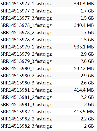
先看这几个1/2/3都是什么部分：

cd /public/home/GENE_proc/wth/GSE174367/fastq/
for fq in SRR14513977_{1,2,3}.fastq.gz; do
  echo "===== $fq ====="
  zcat "$fq" | awk '
    NR%4==2 && ++n<=200000 {len[length($0)]++}
    END{
      for (l in len) print l, len[l]
    }' | sort -n
  echo
done

• SRR14513977_1.fastq.gz：都是8bp，是sample index read
• 正常来讲另外两个应该一个是28bp，另一个是90-100bp，但很神奇的是另外两个都是100bp
• GPT说是没切成28bp的形式，而是原始格式，需要自己看一下哪个是barcode+UMI，哪个是cDNA

import gzip
import sys
import math
from collections import Counter
N = 200000
MAX_POS = 40
def rc(seq):
    comp = str.maketrans("ACGTN", "TGCAN")
    return seq.translate(comp)[::-1]
def iter_seqs(fq, n=N):
    count = 0
    with gzip.open(fq, "rt") as f:
        for i, line in enumerate(f):
            if i % 4 == 1:
                yield line.strip()
                count += 1
                if count >= n:
                    break
def entropy(counter):
    total = sum(counter.values())
    if total == 0:
        return 0.0
    h = 0.0
    for v in counter.values():
        p = v / total
        h -= p * math.log2(p)
    return h
def load_whitelist(path):
    wl = set()
    opener = gzip.open if path.endswith(".gz") else open
    with opener(path, "rt") as f:
        for line in f:
            wl.add(line.strip())
    return wl
def analyze_fastq(fq, whitelist=None):
    seqs = list(iter_seqs(fq, N))
    if not seqs:
        print(f"\n===== {fq} =====")
        print("No reads found")
        return
    lens = Counter(map(len, seqs))
    dom_len, dom_n = lens.most_common(1)[0]
    print(f"\n===== {fq} =====")
    print(f"sampled reads: {len(seqs)}")
    print("length distribution:")
    for l, c in sorted(lens.items()):
        print(f"  {l} bp\t{c}")
    print(f"dominant length: {dom_len} bp ({dom_n/len(seqs):.2%})")
    p16 = [s[:16] for s in seqs if len(s) >= 16]
    p28 = [s[:28] for s in seqs if len(s) >= 28]
    c16 = Counter(p16)
    c28 = Counter(p28)
    print(f"unique first16: {len(c16)} / {len(p16)} ({len(c16)/len(p16):.2%})")
    print(f"unique first28: {len(c28)} / {len(p28)} ({len(c28)/len(p28):.2%})")
    print("top 10 first16:")
    for s, c in c16.most_common(10):
        print(f"  {c}\t{s}")
    print("top 10 first28:")
    for s, c in c28.most_common(10):
        print(f"  {c}\t{s}")
    if whitelist is not None:
        hit = sum((x in whitelist) for x in p16)
        hit_rc = sum((rc(x) in whitelist) for x in p16)
        print(f"whitelist hit rate (first16): {hit/len(p16):.2%}")
        print(f"whitelist hit rate (reverse-complement first16): {hit_rc/len(p16):.2%}")
    tails = [s[28:60] for s in seqs if len(s) >= 60]
    polyA = sum(("AAAAAAAAAAAA" in x) for x in tails)
    polyT = sum(("TTTTTTTTTTTT" in x) for x in tails)
    print(f"reads with >=12A in pos29-60: {polyA/len(tails):.2%}")
    print(f"reads with >=12T in pos29-60: {polyT/len(tails):.2%}")
    pos_counts = [Counter() for _ in range(MAX_POS)]
    for s in seqs:
        for i, b in enumerate(s[:MAX_POS]):
            pos_counts[i][b] += 1
    print("\nPer-cycle summary (first 40 cycles):")
    print("pos\tmajor_base\tmajor_frac\tentropy\tA\tC\tG\tT\tN")
    for i, cnt in enumerate(pos_counts, start=1):
        total = sum(cnt.values())
        if total == 0:
            continue
        major_base, major_n = cnt.most_common(1)[0]
        A = cnt.get("A", 0) / total
        C = cnt.get("C", 0) / total
        G = cnt.get("G", 0) / total
        T = cnt.get("T", 0) / total
        Nn = cnt.get("N", 0) / total
        H = entropy(cnt)
        print(f"{i}\t{major_base}\t{major_n/total:.3f}\t{H:.3f}\t{A:.3f}\t{C:.3f}\t{G:.3f}\t{T:.3f}\t{Nn:.3f}")
if __name__ == "__main__":
    if len(sys.argv) < 3:
        print("Usage: python inspect_10x_cb_umi.py whitelist.txt.gz file1.fastq.gz file2.fastq.gz ...")
        sys.exit(1)
    wl = load_whitelist(sys.argv[1])
    for fq in sys.argv[2:]:
        analyze_fastq(fq, wl)

cd /public/home/GENE_proc/wth/GSE174367/fastq/
python ../inspect_10x_cb_umi.py \
  /public/home/wangtianhao/Desktop/STAR_ref/whitelist/3M-february-2018.txt \
  SRR14513977_2.fastq.gz \
  SRR14513977_3.fastq.gz

最后算出来_2的前16bp对whitelist的命中率高达96%，并且它的unique first16只有14.52%，但加上12bp以后，unique first28达到91.62%，说明前16位是barcode，后12bp是UMI

先跑一个测试：

module load miniconda3/base
conda activate STAR
cd /public/home/GENE_proc/wth/GSE174367/
STAR \
    --runMode alignReads \
    --runThreadN 8 \
    --genomeDir /public/home/wangtianhao/Desktop/STAR_ref/hg38/ \
    --readFilesIn fastq/SRR14513977_3.fastq.gz fastq/SRR14513977_2.fastq.gz \
    --readFilesCommand zcat \
    --outFileNamePrefix star_test/SRR14513977 \
    --soloType CB_UMI_Simple \
    --soloCBstart 1 \
    --soloCBlen 16 \
    --soloUMIstart 17 \
    --soloUMIlen 12 \
    --soloBarcodeReadLength 0 \
    --soloCBwhitelist /public/home/wangtianhao/Desktop/STAR_ref/whitelist/3M-february-2018.txt \
    --soloFeatures GeneFull \
    --clipAdapterType CellRanger4 \
    --soloCellFilter EmptyDrops_CR \
    --soloCBmatchWLtype 1MM_multi_Nbase_pseudocounts \
    --soloUMIfiltering MultiGeneUMI_CR \
    --soloUMIdedup 1MM_CR

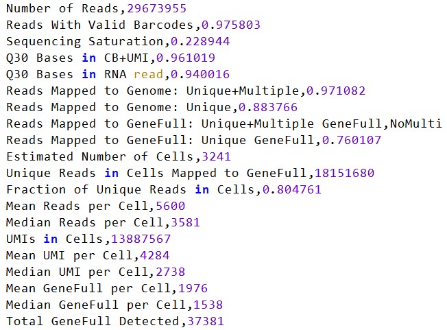
再跑一个完整的样本（包含多个SRR）

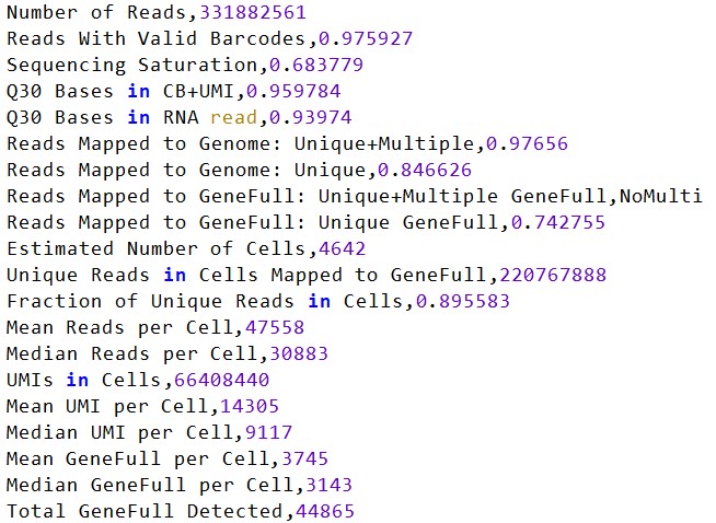
这个GSM5292838在作者的统计表里有4605个细胞（我的有4642个细胞），可以说是完全吻合，由此这个计数参数应该是没有什么问题的

总结：

• 6w多个细胞，来自18个样本，虽然GEO数据库中有19个，但根据论文的补充材料，作者只使用了其中的18个，实测可能是因为差的那个测序质量不太好（nCount_RNA比较低）
• 测序深度较深，nCount_RNA/nFeature_RNA较大（虽然细胞数只有前组数据的1/3，但fastq文件大小却接近3/4）
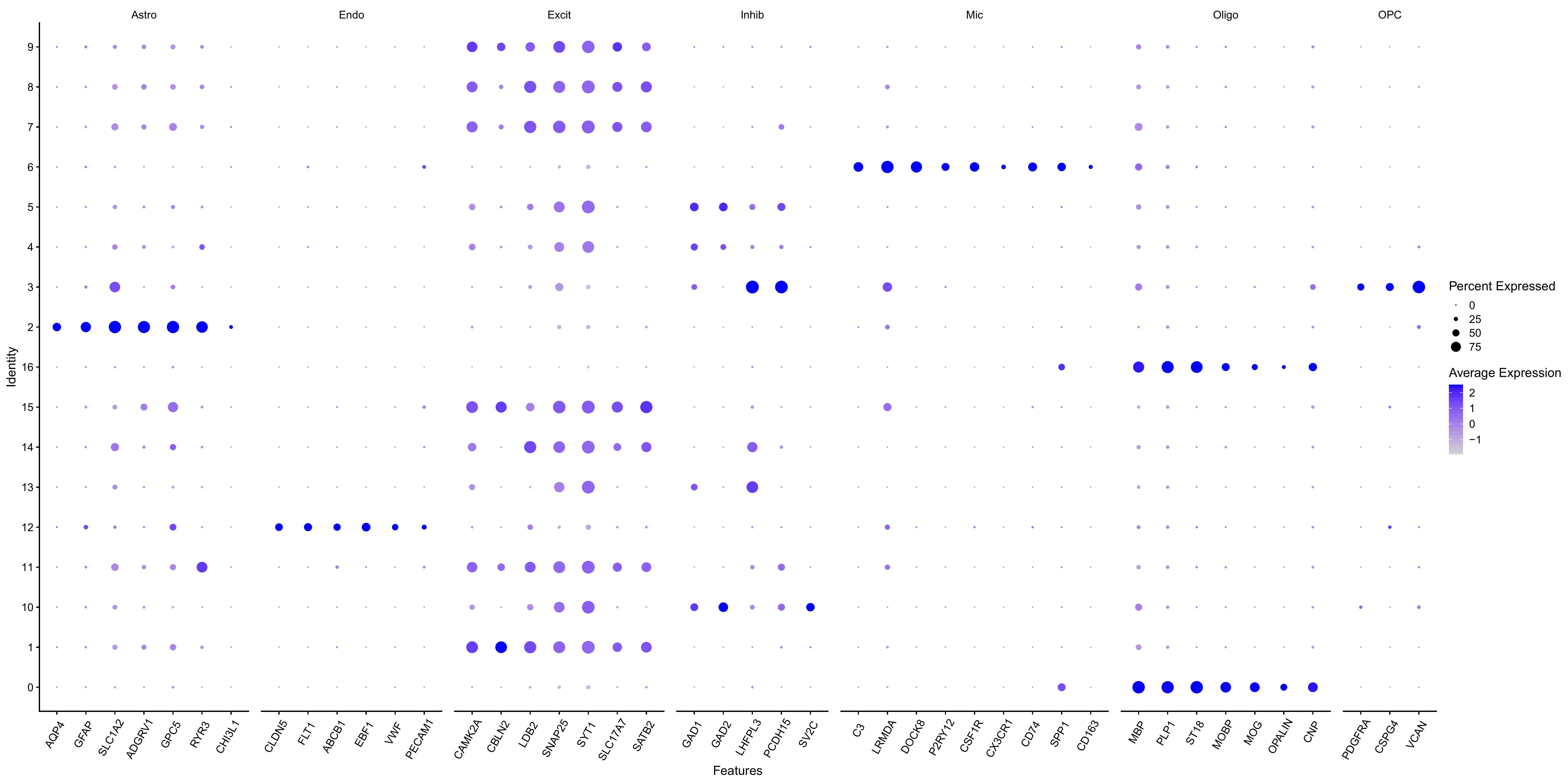
• 在该数据对应的论文中，作者分了7种细胞类型，在之前的6种基础上，增加了“少突胶质前体细胞”(OPC, oligodendrocyte progenitor cells)——具有分化生成成熟少突胶质细胞的能力，在大脑早期发育的髓鞘形成过程中起重要作用

hERV ~ gene

主要思路：

• 在细胞类型层面做hERV~gene共表达分析（不在亚群层面上）：构建共表达网络，把网络中邻近的基因进行功能富集
• 在各细胞类型里找hERV特异表达的亚群，聚焦到某些亚群中高表达的subfamilies做一些定性分析：看这个亚群中特异表达的hERV在共表达网络中连接的基因，对比这个亚群与其它亚群的差异表达基因，看是否与AD有关
• 验证hERVK与TLR8表达相关（先所有细胞，再看细胞类型），参照那篇论文，为下一步hERV位点分析选择位点？

共表达网络test

在之前的代码中，我做的是一个hERV和一个gene的相关性或线性拟合，现在想做一下网络层面的关系：

• 在某个大细胞类型里，哪些基因会一起变化、组成模块，这些模块和hERV是否相关
• 某个hERV高表达亚群里，究竟激活了哪一类网络程序
• WGCNA/hdWGCNA（用于单细胞数据的WGCNA）：先用表达相关性构建加权网络，再把高度共表达的基因聚成模块，用模块特征值去和外部性状做关联
• 在构建完网络之后，可以在某个和hERV明显相关的模块里，再去找和这个hERV相关性最高的基因（一个hERV和一个gene的线性拟合）

方案1：先用基因构建共表达网络，再把hERV当作外部性状去挂到网络上（GPT推荐）

• 在细胞大类中，单独构建基因的共表达网络，得到若干个基因模块
  • 选在该细胞类型中有一定表达比例的基因
• 把hERV的表达和模块特征值做关联
  • 选定一些trait：hERV家族表达量、AD/NC等
  • 模块特征值和trait的相关分析，画热图
• 找到和某个hERV家族显著相关的模块
  • 例如某个模块和hERVK表达显著相关，同时和AD状态相关，那么这个模块就是一个很有价值的“hERV-AD关联模块”
• 后续对这些模块进行亚群级别的分析（具体方法在方案1中有讲）

方案2：把hERV当成普通基因作为网络节点直接参与建网

• 取网络中与hERV相邻的一些基因进行亚群级别的分析
• GPT不推荐，说是会存在一些问题：
  • hERV家族数量远少于基因，且表达更稀疏
  • hERV节点本身不能直接做GO
  • 在WGCNA时，hERV要和普通基因一同作为feature进行标准化，这样就和之前单独标准化的思路不同，不过考虑到hERV表达量很低，影响也许不大？

采用哪种方案比较好：

• 方案1会更好解释家族水平hERV
• 方案2看起来更适合探讨位点级别的局部网络

---

共表达网络的5个对象：

• 节点(node)：通常是gene
• 边(edge)：表示两个基因在同一大细胞类型内、在不同样本/细胞中的表达是否同步变化
• 模块(module)：一群彼此更紧密共表达的基因，往往对应某种生物过程
• 模块特征值(module eigengene, ME)：本质上是模块表达矩阵的一个总结量，可以理解成“这个模块整体表达水平的代表值”，用于回答“这个模块在AD中是否表达更高”等问题
• hub gene：模块里连接度高、最核心的基因，通常是模块的代表基因或关键解释点。hdWGCNA里常用kME去衡量这种模块内连接性

共表达网络其它的一些专业名词：

• metacell：把若干个彼此相近、而且来自同一分组里的单细胞做平均，得到一个更稳定的小样本单元，如果设置为group.by = c("wgcna_celltype", "orig.ident")就是先限制在同一个大细胞类型里，再限制在同一个sample里，然后在这些细胞里找相近细胞做平均。既保留了细胞类型特异性，又降低了单细胞水平分析的噪声
• trait：和模块做关联的外部变量——某个module的整体表达水平，是否随着某个trait变化
• soft power：WGCNA不会直接把基因之间的相关性（0.2/0.5/0.8这种）当网络中边的值，而是会加一个指数soft power，决定要把“高相关”和“低相关”的差距拉大到什么程度。这个指数变换可以把弱相关压小、强相关放大，如果power过小，网络对强弱相关的区分就不够；power慢慢增大，使网络结构更接近WGCNA想要的“scale-free”特征；如果power过大，整体网络会越来越稀，很多真实联系可能被压掉
• scale-free：无标度，指的是一种网络结构——大多数节点连接很少，只有少数节点连接特别多，也就是网络里会有少量枢纽节点(hub gene)，而不是每个节点都连得差不多
• TOM：拓扑重叠矩阵(Topological Overlap Matrix)，不是只看两个基因自己相关不相关，而是进一步看它们是不是拥有很多共同邻居
  • 基因A和基因B直接相关，当然说明它们可能有关
  • 但如果A和B不仅彼此相关，而且还都和C、D、E一起相关，那说明它们在网络中的“位置”也很像
  • 这种“共同邻居很多”的关系，TOM会给更高分

  所以它比单纯相关性更稳一些，因为它用了局部网络结构信息，而不是只看一条边

方案1

构建纯gene的共表达网络：

herv_assay <- "HERV_family"
celltype_name <- "Oligo"
herv_traits <- c("HERV3-int", "HERVH-int", "HERVE-int", "HERVK-int", "HERVK3-int", "HERVK9-int", "HERVK11-int", "HERVK13-int", "HERVK14-int", "HERVK22-int")
DefaultAssay(seu) <- "RNA"
seu$AD_binary <- ifelse(seu$group == "AD", 1, 0)
# 把trait写入metadata
mat <- LayerData(seu, assay = herv_assay, layer = "data")[herv_traits, , drop = FALSE]
mat <- t(as.matrix(mat))
colnames(mat) <- paste0("herv_", make.names(herv_traits))
seu <- AddMetaData(seu, metadata = as.data.frame(mat))
# SetupForWGCNA
seu <- SetupForWGCNA(  # 运行时间几分钟
  seu,
  gene_select = "fraction",
  fraction = 0.05,  # 过滤掉表达比例<5%的基因
  assay = "RNA",
  wgcna_name = "gene_net"
)
# 构建metacell（按样本分开）
seu <- MetacellsByGroups(  # 运行时间20min，需要10G+内存
  seurat_obj = seu,
  group.by = c("celltype", "orig.ident"),
  ident.group = "celltype",
  assay = "RNA",
  layer = "data",
  reduction = "pca",
  dims = 1:30,
  k = 25,
  max_shared = 10,
  min_cells = 50,
  mode = "average",
  wgcna_name = "gene_net"
)
seu <- NormalizeMetacells(seu, wgcna_name = "gene_net")
# 设置网络表达矩阵
seu <- SetDatExpr(  # 运行时间几分钟
  seu,
  group_name = celltype_name,
  group.by = "celltype",
  use_metacells = TRUE,
  assay = "RNA",
  layer = "data",
  wgcna_name = "gene_net"
)
# 选soft power
seu <- TestSoftPowers(  # 运行时间几分钟
  seu,
  networkType = "signed",
  wgcna_name = "gene_net"
)
power_table <- GetPowerTable(seu)
soft_power <- power_table$Power[which(power_table$SFT.R.sq >= 0.8)[1]]
if (is.na(soft_power)) {
  soft_power <- power_table$Power[which.max(power_table$SFT.R.sq)]
}
plot_list <- PlotSoftPowers(seu)
pdf(file.path(res_dir, "oligo_soft_power.pdf"), width = 16, height = 16)
p <- patchwork::wrap_plots(plot_list, ncol = 2)
print(p)
dev.off()
save(seu, soft_power, herv_traits, file = file.path(res_dir, "oligo_WGCNA_before_ConstructNetwork.RData"))
# 构建网络
seu <- ConstructNetwork(  # 运行时间20min，需要50G+内存
  seu,
  soft_power = soft_power,
  networkType = "signed",
  tom_name = "seu_TOM",
  wgcna_name = "gene_net"
)
# 计算module eigengenes
seu <- ModuleEigengenes(  # 运行时间20min，需要50G+内存
  seu,
  group.by.vars = "orig.ident",
  assay = "RNA",
  wgcna_name = "gene_net"
)
# module~trait关联
trait_cols <- c(
  paste0("herv_", make.names(herv_traits)),
  "AD_binary"
)
seu$celltype <- factor(seu$celltype)
seu <- ModuleTraitCorrelation(
  seu,
  traits = trait_cols,
  group.by = "celltype",
  wgcna_name = "gene_net"
)
mt <- GetModuleTraitCorrelation(seu)
# 结果
View(mt$cor)  # 相关系数
View(mt$fdr)  # FDR校正后p值
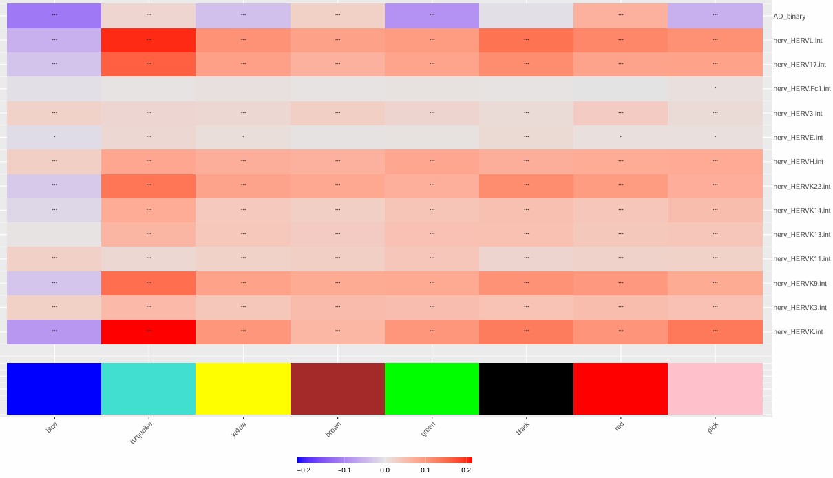
pdf(file.path(res_dir, "oligo_trait_corr.pdf"), width = 16, height = 16)
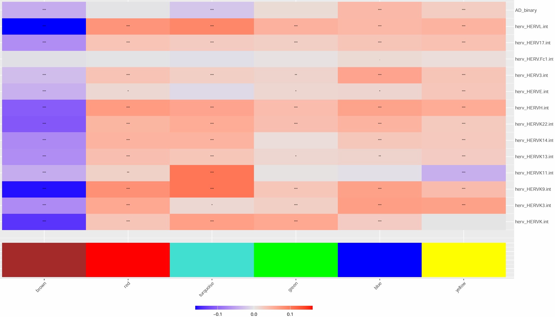
p <- PlotModuleTraitCorrelation(seu, label = "fdr", label_symbol = "stars")
print(p)
dev.off()

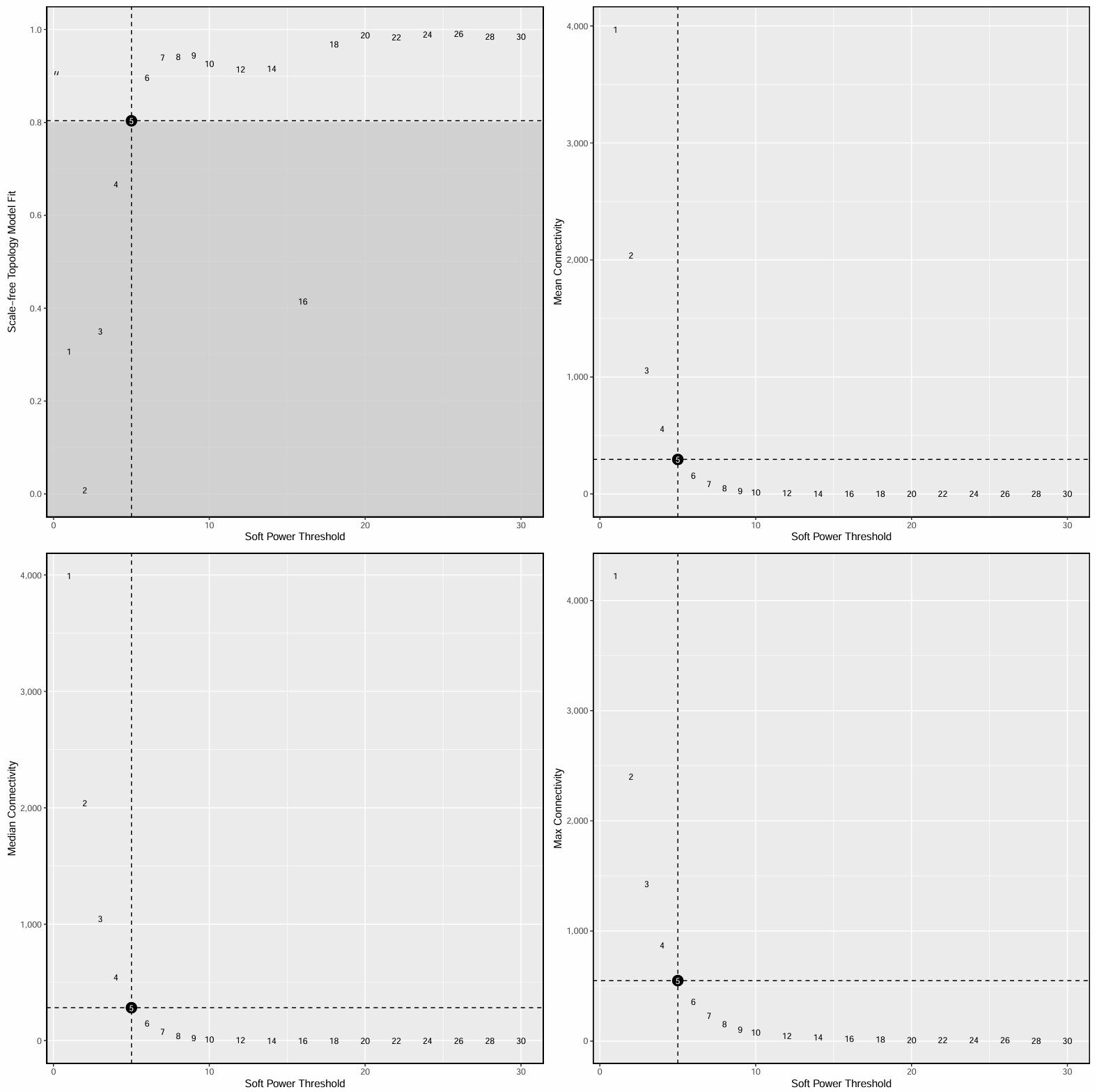
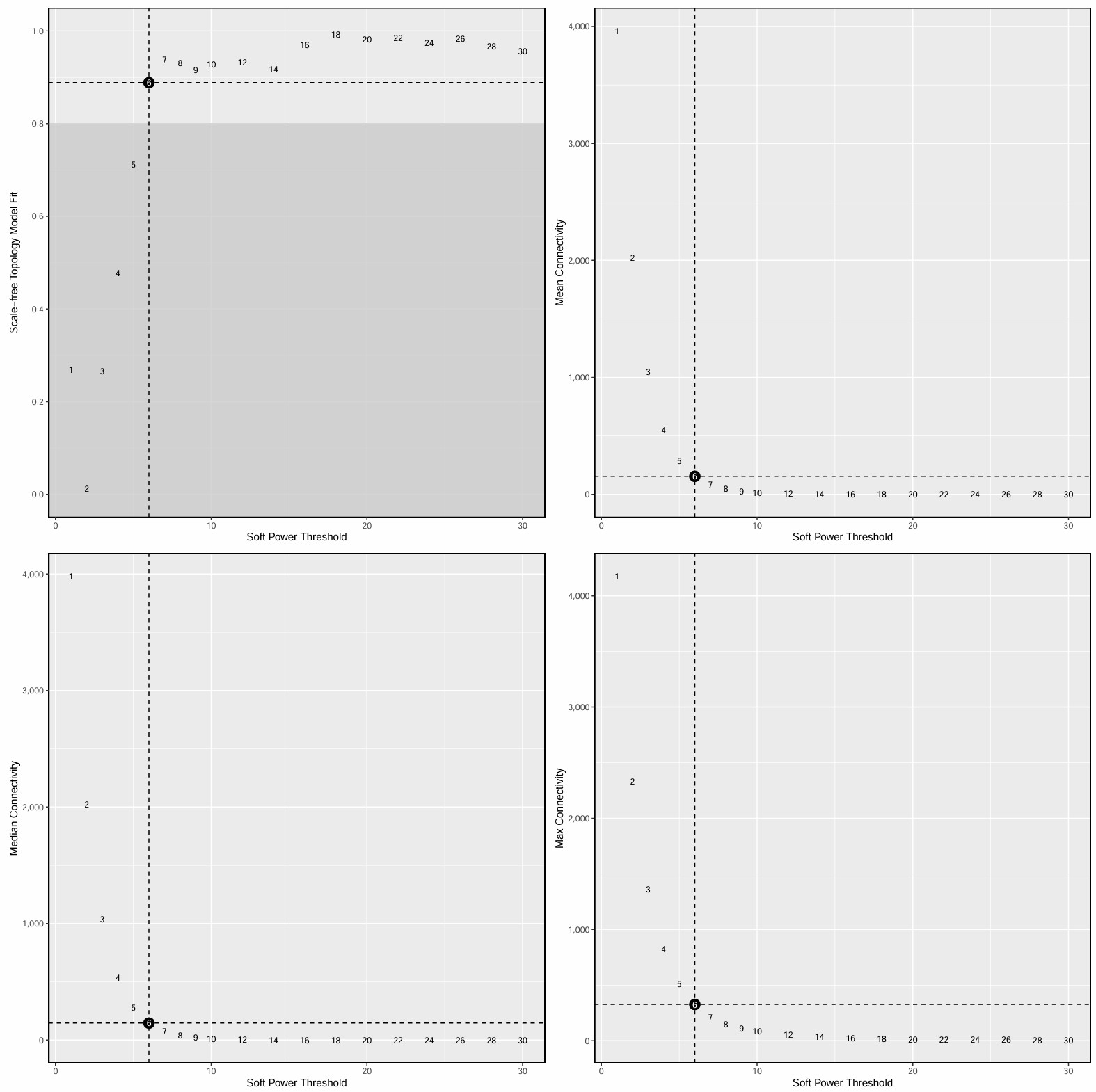
• 横轴是power，纵轴是scale-free topology model fit(signed R²)，常取第一个让R²达到设定阈值（比如0.8左右）的power。如果数据本身比较噪、样本数少、或者是mixed network，达不到理想值也很常见，此时就选一个相对合理、且曲线已经进入平台区的power
• 横轴是power，纵轴是平均连接度(Mean connectivity)，在“结构合理”和“不要过稀”之间找平衡
• 在这个结果中，power=5是一个比较合适的折中点，SFT.R.sq已达到阈值，连通性还保留得可以

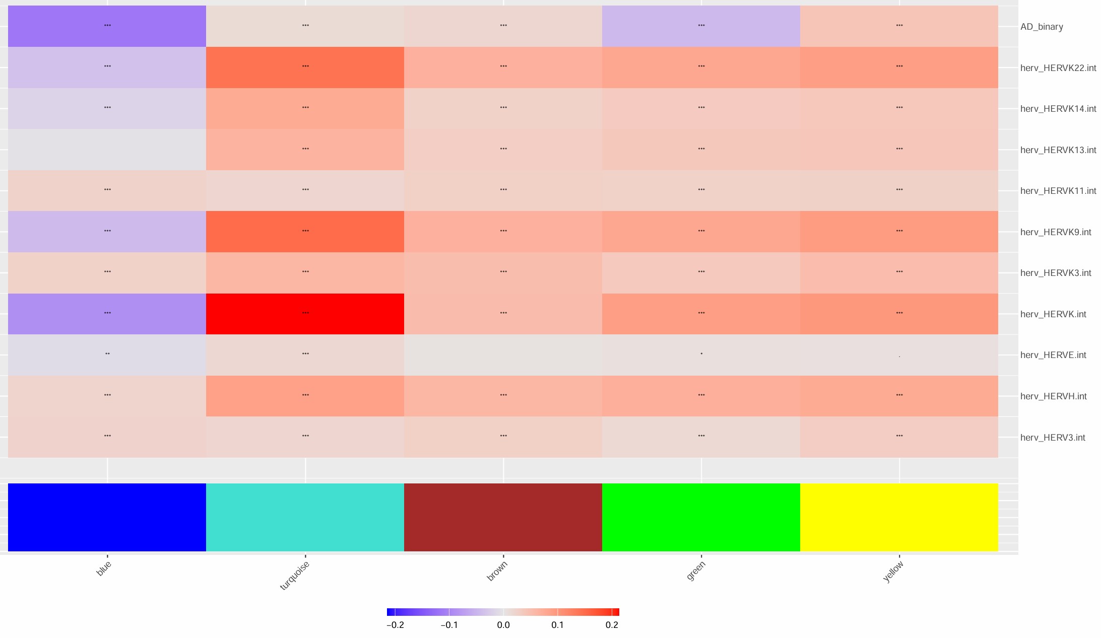
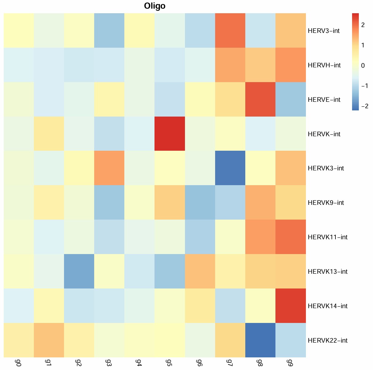
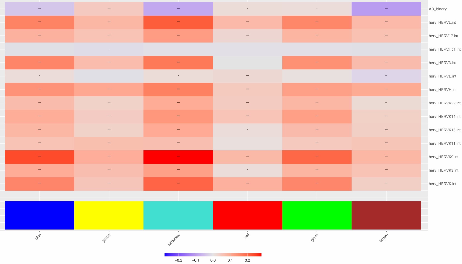
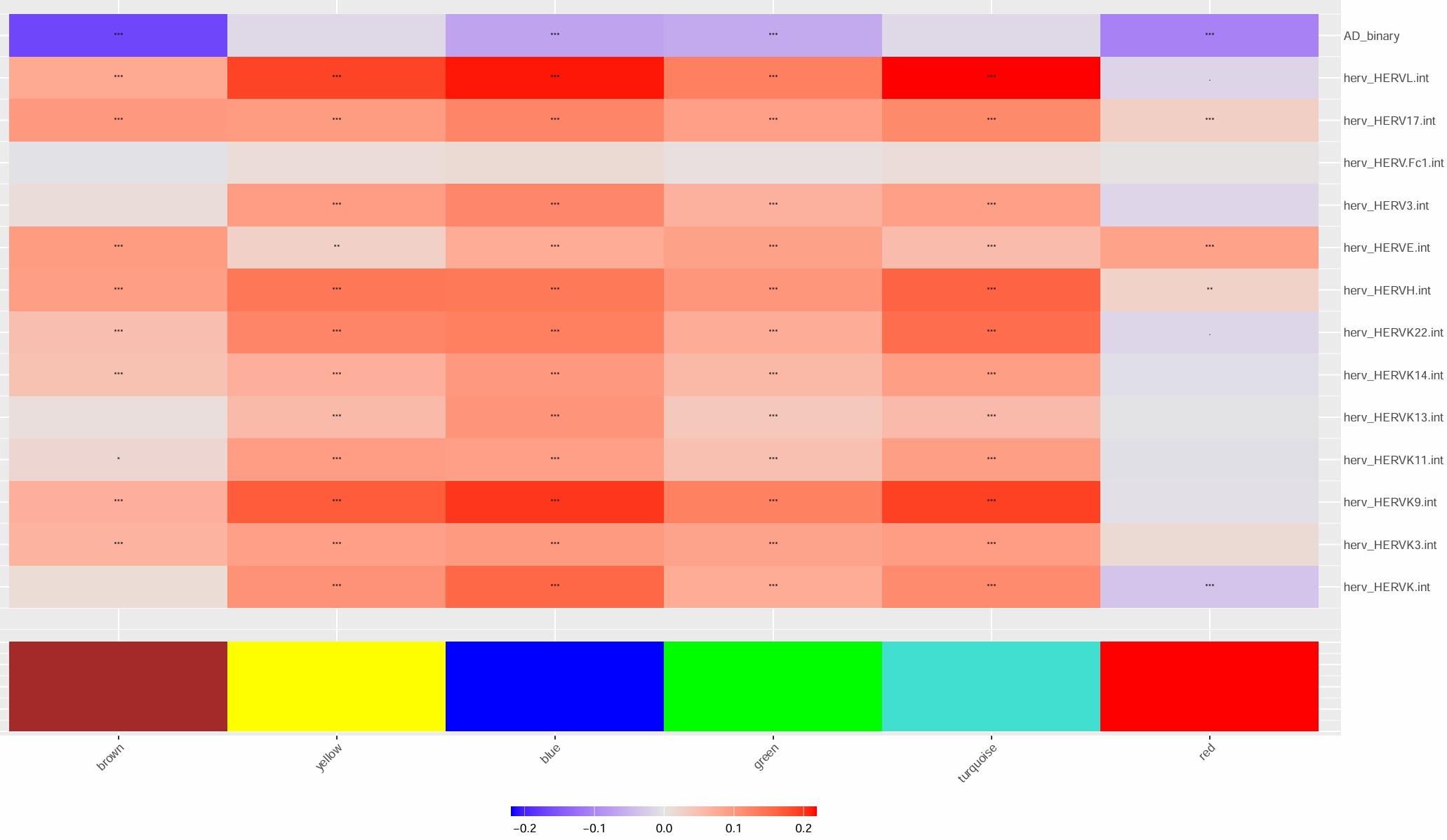
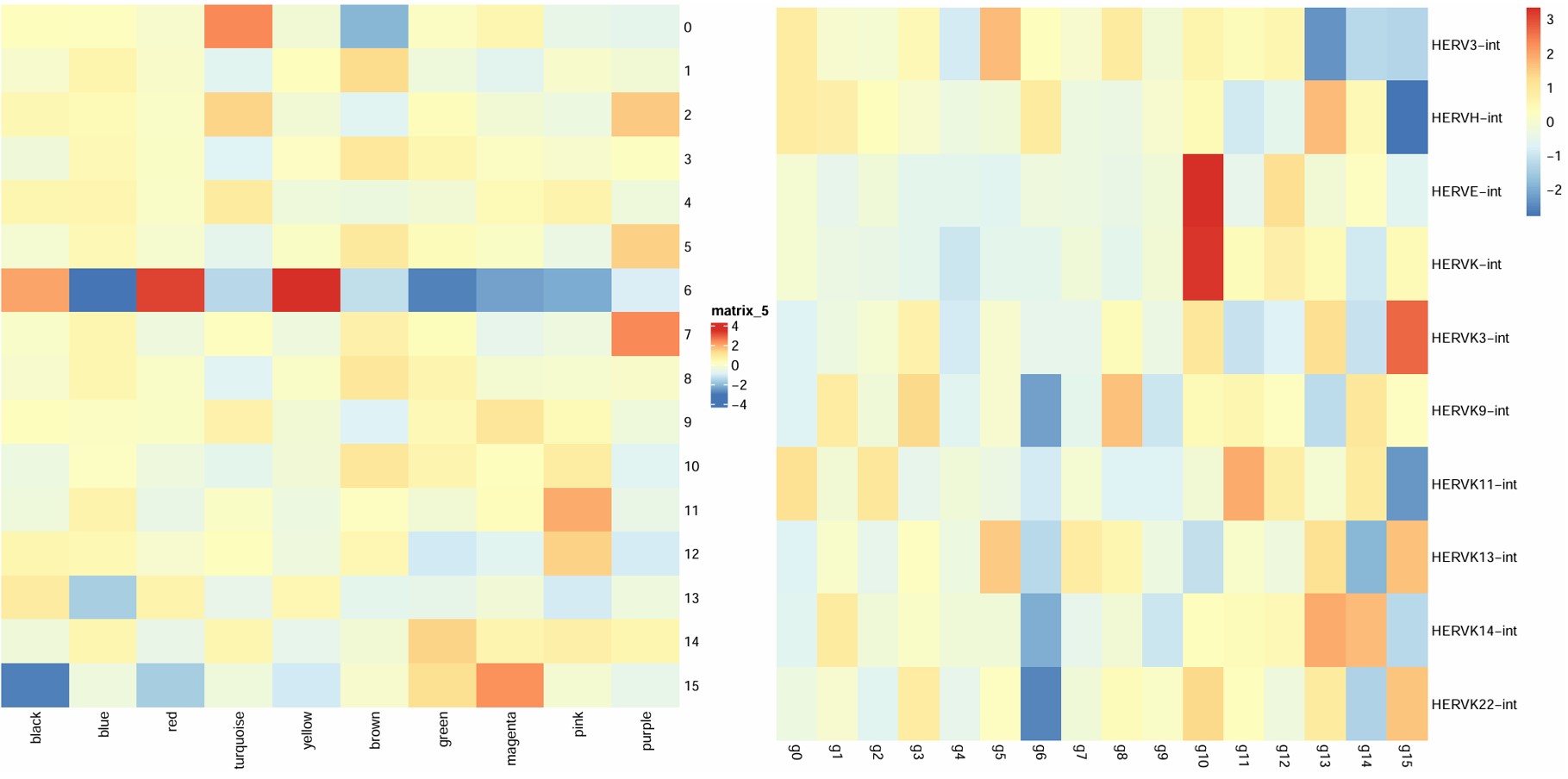
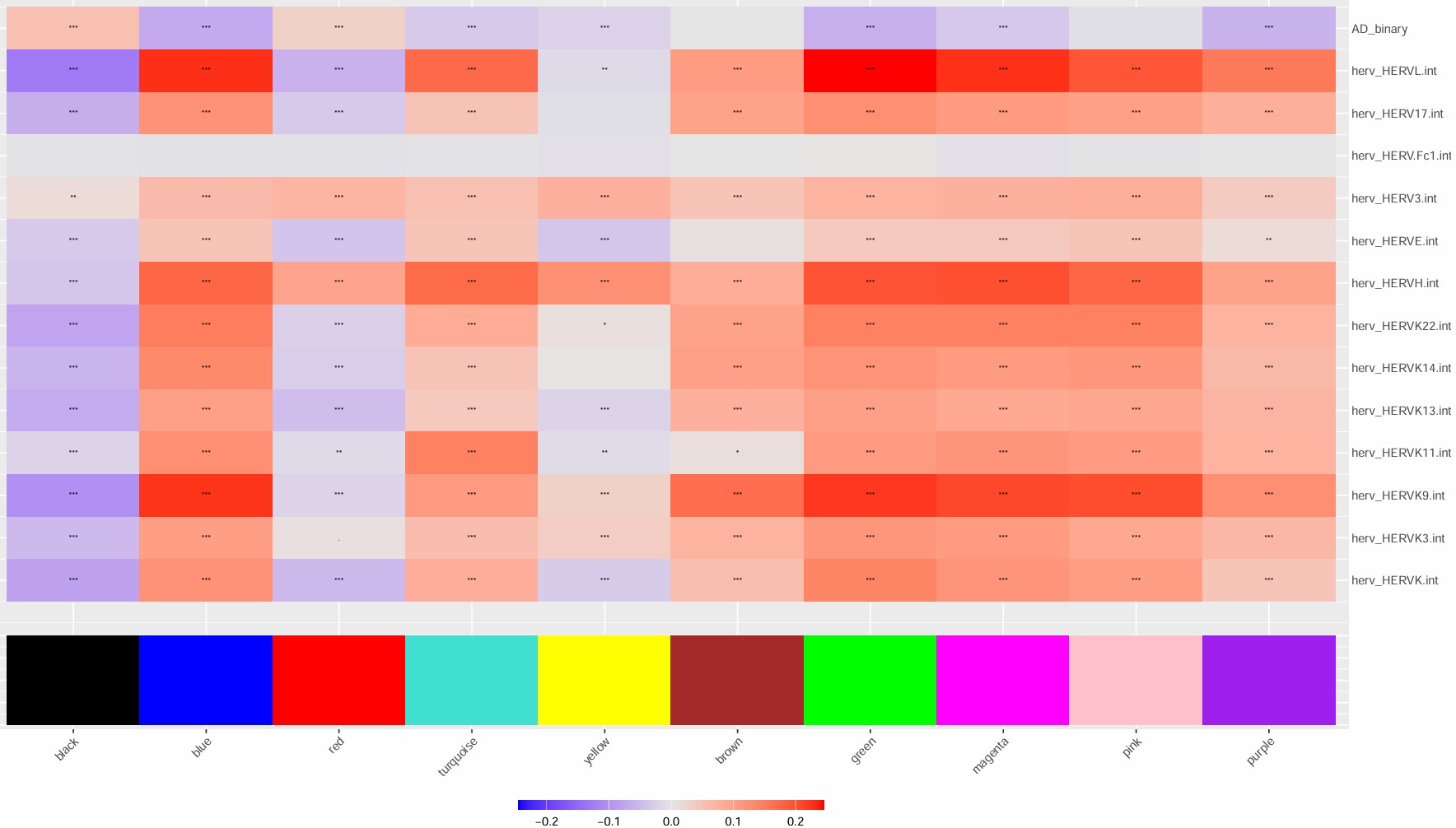
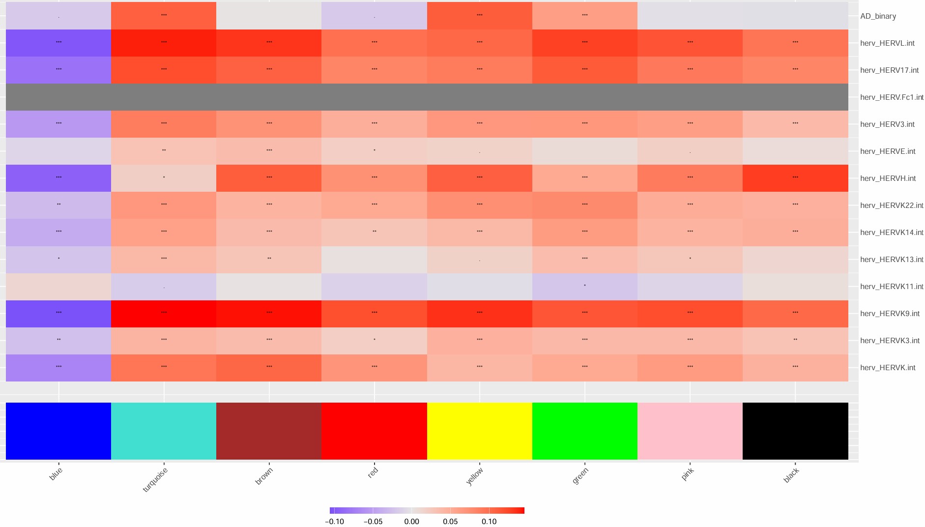
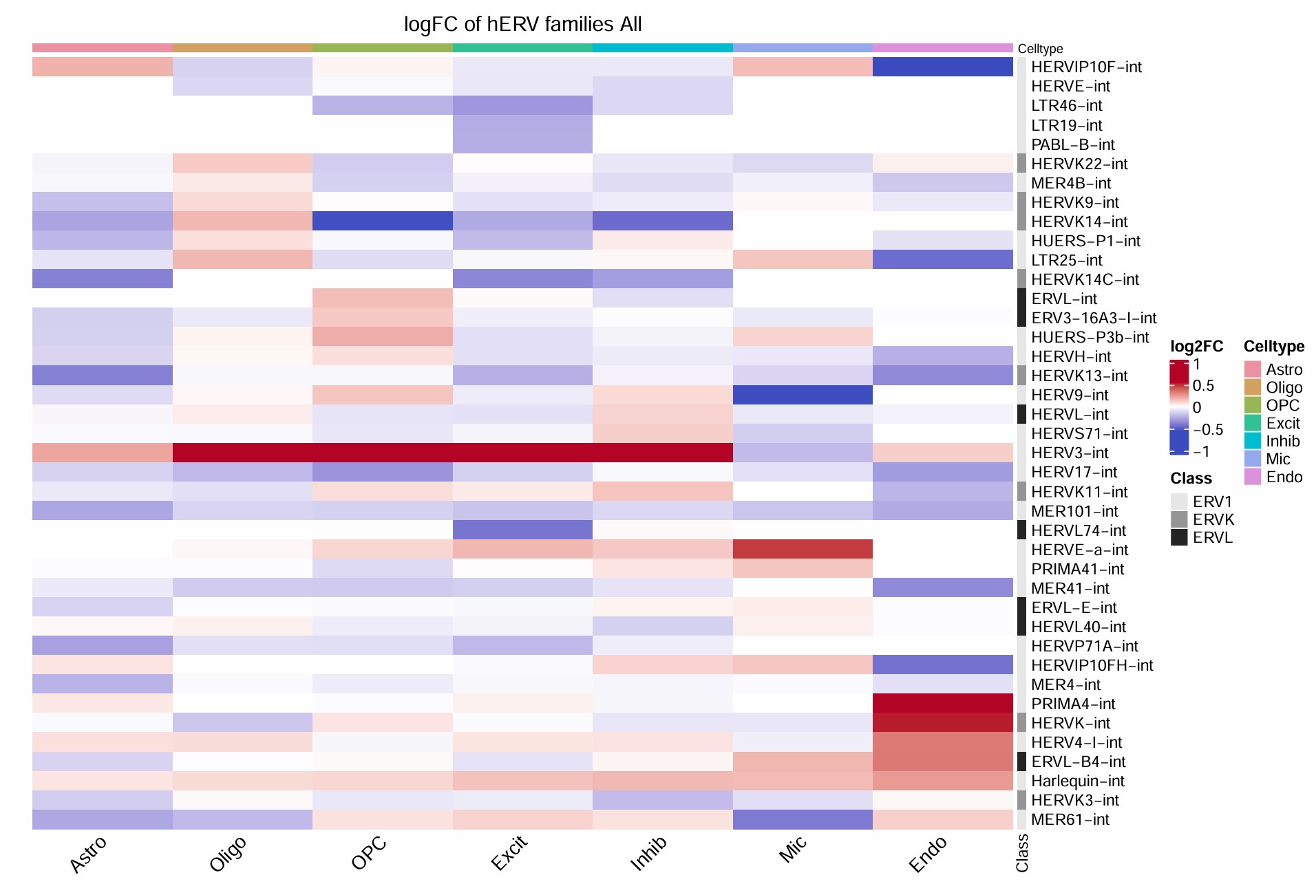
• turquoise模块最值得关注，几乎所有的hERV都是正相关
• blue模块和很多hERV是反向的
• 比较意外的是，这几个模块和AD的相关性竟然不是很高
• 不过总体来说相关度不算特别大，几乎都是-0.2~0.2的水平，

从gene network里提取“和某个hERV trait相关的模块”和hub genes

# 计算kME/hub genes
seu <- ModuleConnectivity(
  seu,
  group.by = "celltype",
  group_name = celltype_name,
  assay = "RNA",
  wgcna_name = "gene_net"
)
save(seu, file = file.path(res_dir, "oligo_WGCNA.RData"))
# 目标hERV
trait_keep <- grep("^herv_", rownames(GetModuleTraitCorrelation(seu)$cor$all_cells), value = TRUE)
n_hubs <- 50  # 每个模块取多少个hub genes
pick_col <- function(df, candidates) {
  x <- intersect(candidates, colnames(df))
  if (length(x) == 0) stop("找不到列: ", paste(candidates, collapse = ", "))
  x[1]
}
mat_to_df <- function(mat, value_name) {
  df <- as.data.frame(as.table(as.matrix(mat)), stringsAsFactors = FALSE)
  colnames(df) <- c("module", "trait", value_name)
  df
}
# 选目标模块
fdr_cutoff <- 0.05  # 显著性阈值
cor_cutoff <- 0.05
mt <- GetModuleTraitCorrelation(seu)
cor_df <- mat_to_df(mt$cor$all_cells,  "cor")
fdr_df <- mat_to_df(mt$fdr$all_cells,  "fdr")
sig_tbl <- left_join(cor_df, fdr_df, by = c("module", "trait")) %>%
  # filter(
  #   trait %in% trait_keep,
  #   module != "grey",
  #   !is.na(fdr),
  #   fdr < fdr_cutoff,
  #   abs(cor) >= cor_cutoff
  # ) %>%
  arrange(trait, desc(abs(cor)))
# write.csv(sig_tbl, file.path(res_dir, "oligo_module_trait_significant.csv"), row.names = FALSE)
# target_modules <- unique(sig_tbl$module)
target_modules <- c("turquoise", "blue")  # 手动
# 提取模块基因 + hub genes
modules_df <- GetModules(seu)
hub_df <- GetHubGenes(seu, n_hubs = n_hubs)
gene_col_mod <- pick_col(modules_df, c("gene_name", "gene", "feature"))
module_col_mod <- pick_col(modules_df, c("module", "color"))
gene_col_hub <- pick_col(hub_df, c("gene_name", "gene", "feature"))
module_col_hub <- pick_col(hub_df, c("module", "color"))
# 背景基因设置为网络中的所有基因
universe_genes <- unique(modules_df[[gene_col_mod]])
universe_genes <- universe_genes[!is.na(universe_genes)]
# 只保留显著模块
module_gene_list <- lapply(target_modules, function(m) {
  unique(modules_df[modules_df[[module_col_mod]] == m, gene_col_mod, drop = TRUE])
})
names(module_gene_list) <- target_modules
module_hub_list <- lapply(target_modules, function(m) {
  unique(hub_df[hub_df[[module_col_hub]] == m, gene_col_hub, drop = TRUE])
})
names(module_hub_list) <- target_modules
# 导出模块基因和hub genes
# for (m in target_modules) {
#   write.csv(
#     data.frame(gene = module_gene_list[[m]]),
#     file.path(res_dir, paste0("oligo_genes_", m, ".csv")),
#     row.names = FALSE
#   )
#   write.csv(
#     data.frame(hub_gene = module_hub_list[[m]]),
#     file.path(res_dir, paste0("oligo_hub_genes_", m, ".csv")),
#     row.names = FALSE
#   )
# }
# 汇总结果
module_summary <- data.frame(
  module = target_modules,
  n_genes = sapply(module_gene_list, length),
  n_hubs  = sapply(module_hub_list, length),
  top_hubs = sapply(module_hub_list, function(x) paste(head(x, 10), collapse = ", ")),
  stringsAsFactors = FALSE
)
# write.csv(module_summary, file.path(res_dir, "oligo_module_summary.csv"), row.names = FALSE)
save(target_modules, universe_genes, module_gene_list, sig_tbl, module_hub_list, file = file.path(res_dir, "oligo_target_modules.RData"))

最后发现turquoise有3k多个基因，而blue只有300多个

# GO富集
run_go_one <- function(gene_vec, universe_genes = NULL, ont = "BP") {
  gene_vec <- unique(na.omit(gene_vec))
  if (length(gene_vec) < 10) return(NULL)
  ego <- enrichGO(
    gene          = gene_vec,
    universe      = universe_genes,
    OrgDb         = org.Hs.eg.db,
    keyType       = "SYMBOL",
    ont           = ont,
    pAdjustMethod = "BH",
    pvalueCutoff  = 1,
    qvalueCutoff  = 1,
    readable      = TRUE
  )
  if (is.null(ego) || nrow(as.data.frame(ego)) == 0) return(NULL)
  ego
}
go_list <- lapply(target_modules, function(m) {
  run_go_one(
    gene_vec = module_gene_list[[m]],
    universe_genes = universe_genes,
    ont = "BP"
  )
})
names(go_list) <- target_modules
for (m in target_modules) {
  ego <- go_list[[m]]
  if (is.null(ego)) next
  go_df <- as.data.frame(ego)
  write.csv(
    go_df,
    file.path(res_dir, paste0("GO_BP_", m, ".csv")),
    row.names = FALSE
  )
}
res <- list()
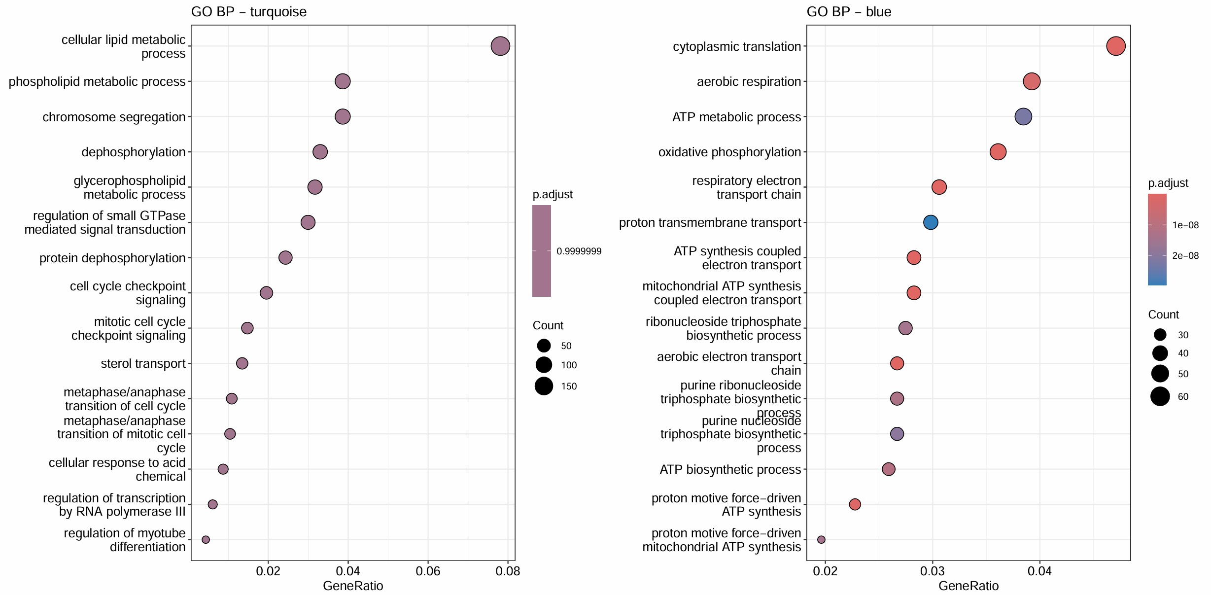
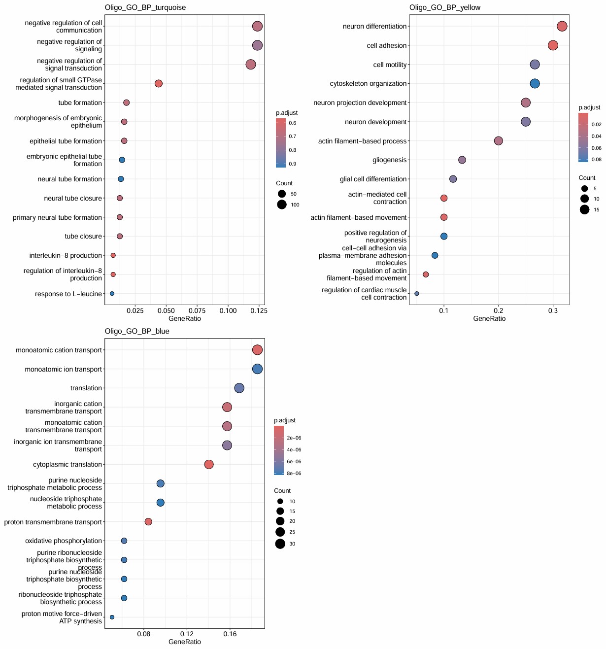
# 画图展示结果
for (m in target_modules) {
  ego <- go_list[[m]]
  if (is.null(ego)) next
  res[[m]] <- dotplot(ego, showCategory = 15) +
    ggtitle(paste0("GO BP - ", m))
}
pdf(file.path(res_dir, "oligo_module_trait_GO_summary.pdf"), width = 15, height = 24)
p <- wrap_plots(res, ncol = 2)
print(p)
dev.off()
# 汇总GO结果
top_go_tbl <- lapply(target_modules, function(m) {
  ego <- go_list[[m]]
  if (is.null(ego)) return(NULL)
  go_df <- as.data.frame(ego)
  go_df <- go_df[order(go_df$p.adjust), ]
  trait_df <- sig_tbl %>%
    filter(trait == m) %>%
    arrange(desc(abs(cor)))
  data.frame(
    module = m,
    trait = paste(trait_df$module, collapse = "; "),
    cor = paste(round(trait_df$cor, 3), collapse = "; "),
    n_gene = length(module_gene_list[[m]]),
    hub_gene = paste(module_hub_list[[m]], collapse = "; "),
    GO = paste(go_df$Description[1:20], collapse = "; "),
    GO_padj = paste(go_df$p.adjust[1:20], collapse = "; "),
    stringsAsFactors = FALSE
  )
}) %>% bind_rows()
write.csv(top_go_tbl, file.path(res_dir, "oligo_module_trait_GO_summary2.csv"), row.names = FALSE)

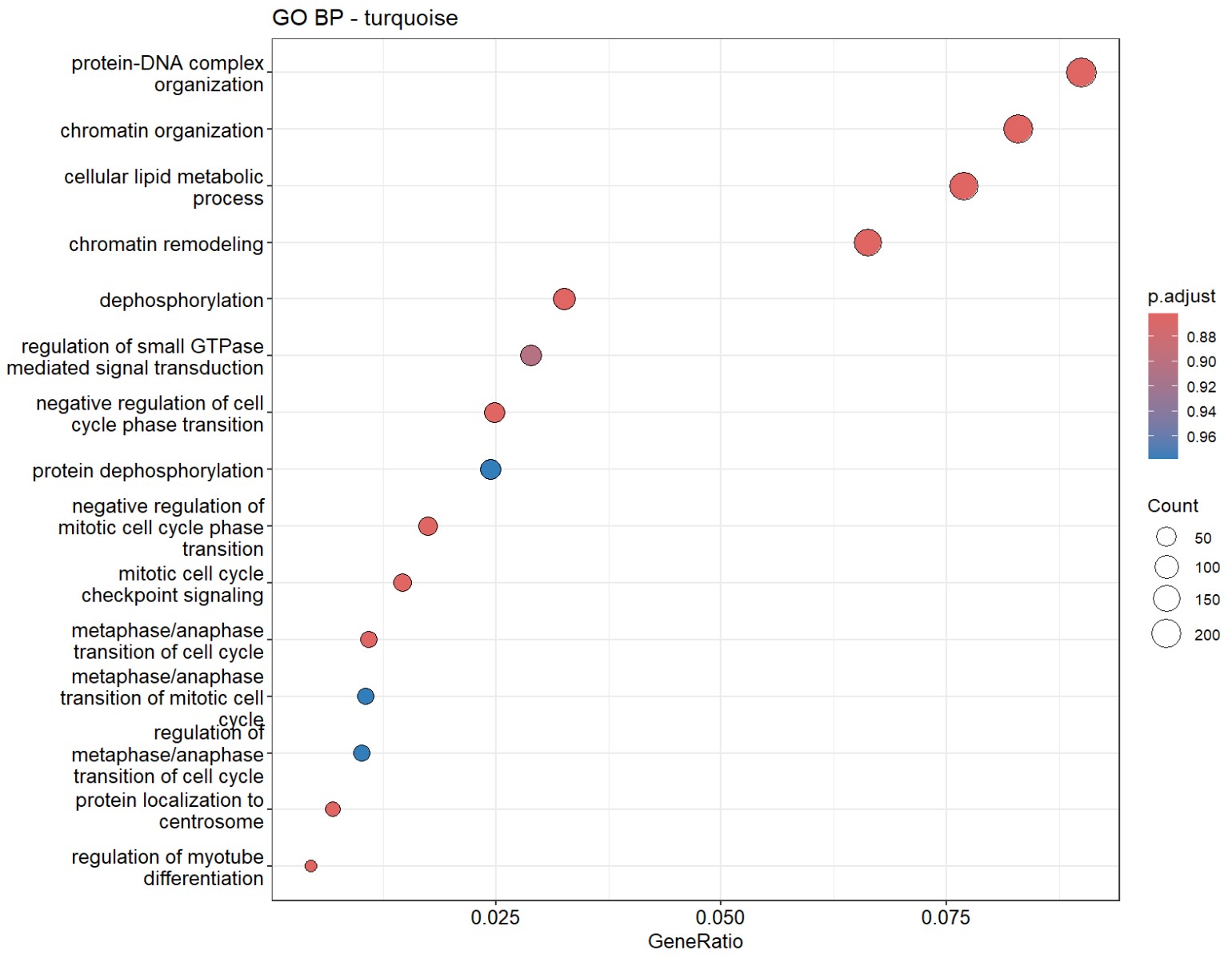
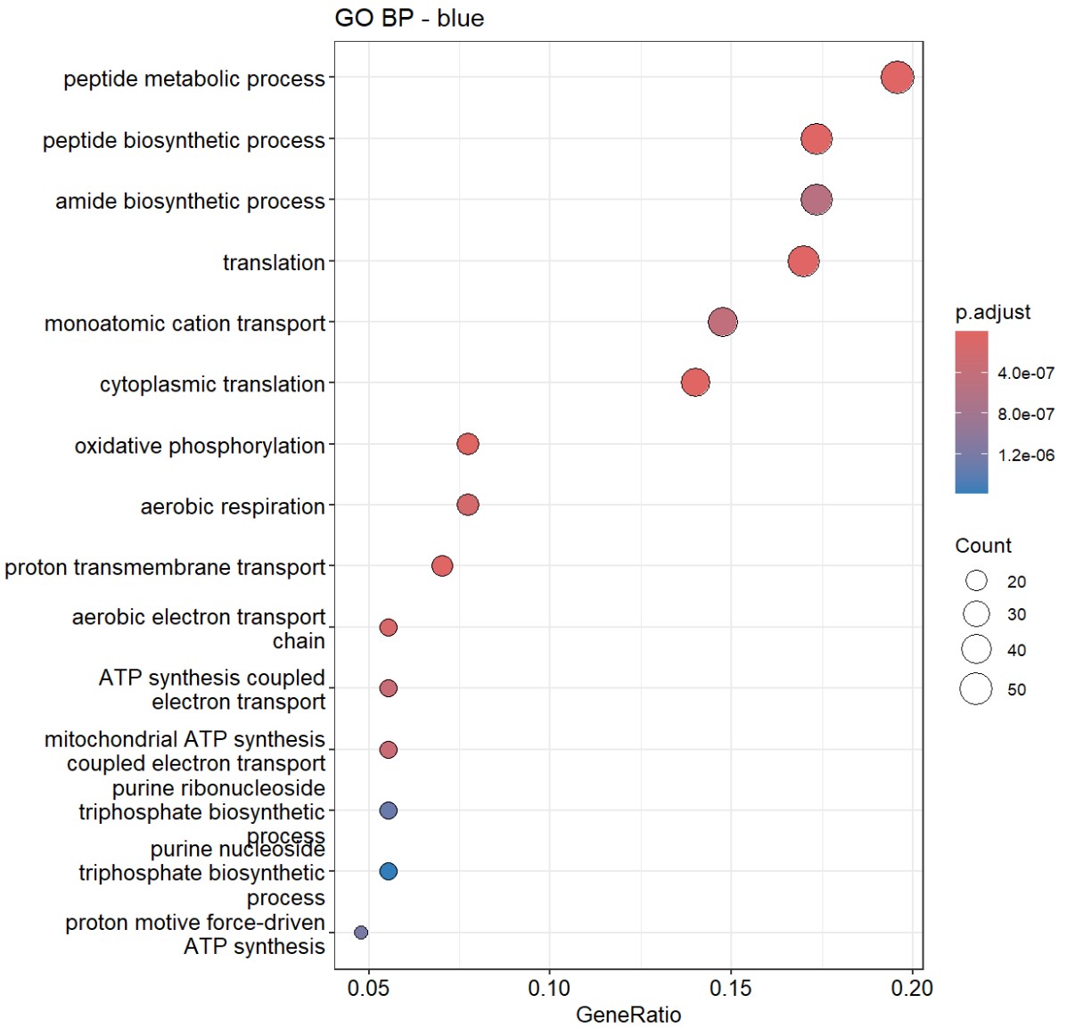
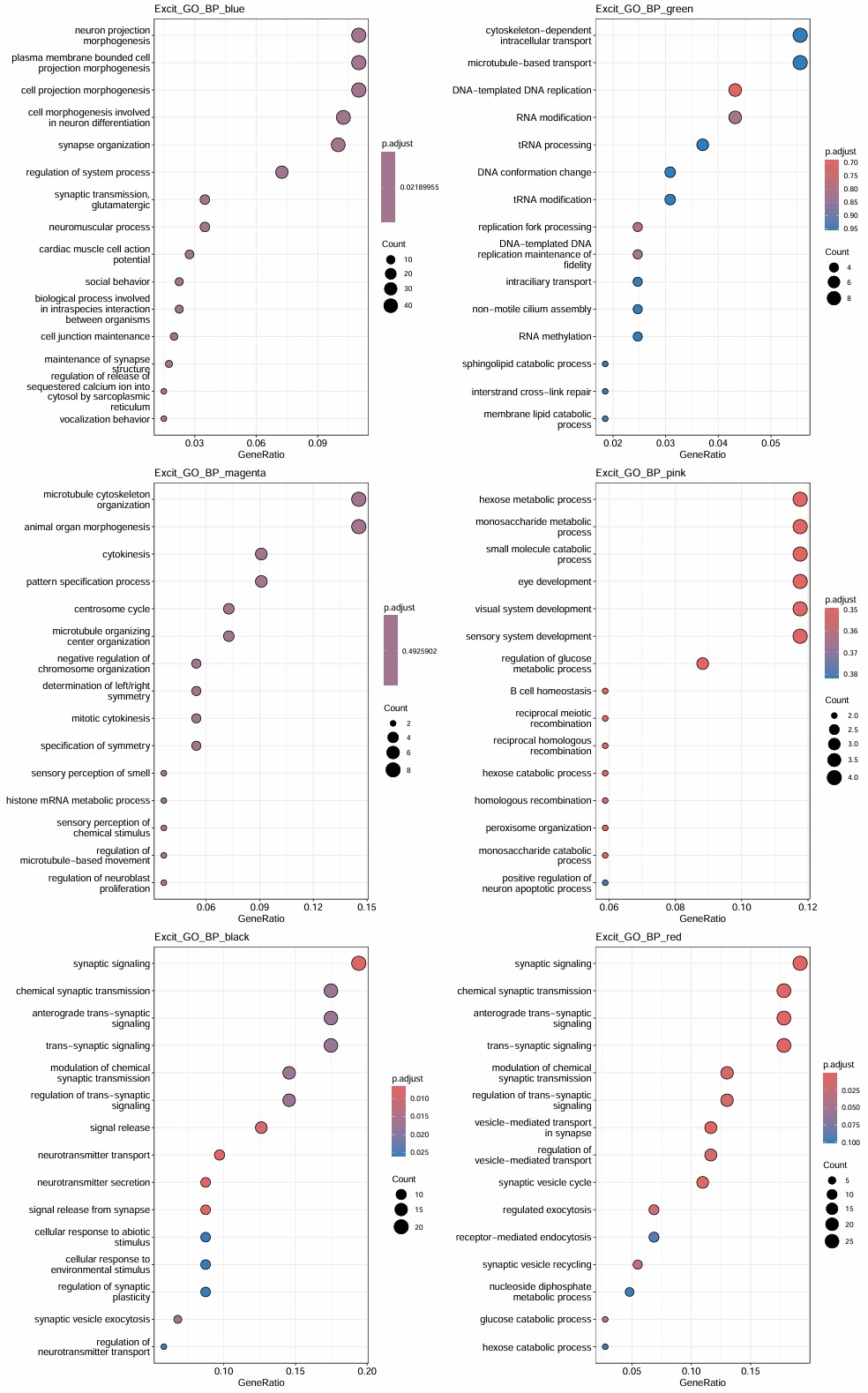
因为turquoise的基因数太多，所以p值就很高。又把两个模块的基因让GPT分析了一下，GPT也觉得turquoise更偏向总体细胞状态，blue的功能同质性更高：

• CNP/OLIG1/NKX6-2/HSPA2/APOD：少突成熟/髓鞘相关
• FTH1/FTL/CRYAB/SELENOP：代谢、应激、铁稳态/保护反应
• 有很多核糖体、线粒体呼吸链相关基因

说明blue很可能对应的是一种代谢活跃/翻译活跃/线粒体活跃/相对成熟稳态的少突程序，而AD和hERV又是负相关，说明在AD或hERV较高的状态下，这套“代谢-翻译-氧化磷酸化”程序是下降的

---

试一试改参数让模块更细一些？改ConstructNetwork中的两个参数：

• fraction = 0.1：过滤掉更多的基因
• minModuleSize = 20：允许更小的模块保留下来
• mergeCutHeight = 0.05：减少相似模块合并

herv_assay <- "HERV_family"
celltype_name <- "Oligo"
herv_traits <- c("HERV3-int", "HERVH-int", "HERVE-int", "HERVK-int", "HERVK3-int", "HERVK9-int", "HERVK11-int", "HERVK13-int", "HERVK14-int", "HERVK22-int")
DefaultAssay(seu) <- "RNA"
seu$AD_binary <- ifelse(seu$group == "AD", 1, 0)
mat <- LayerData(seu, assay = herv_assay, layer = "data")[herv_traits, , drop = FALSE]
mat <- t(as.matrix(mat))
colnames(mat) <- paste0("herv_", make.names(herv_traits))
seu <- AddMetaData(seu, metadata = as.data.frame(mat))
seu <- SetupForWGCNA(
  seu,
  gene_select = "fraction",
  fraction = 0.1,
  assay = "RNA",
  wgcna_name = "gene_net"
)
seu <- MetacellsByGroups(
  seurat_obj = seu,
  group.by = c("celltype", "orig.ident"),
  ident.group = "celltype",
  assay = "RNA",
  layer = "data",
  reduction = "pca",
  dims = 1:30,
  k = 25,
  max_shared = 10,
  min_cells = 50,
  mode = "average",
  wgcna_name = "gene_net"
)
seu <- NormalizeMetacells(seu, wgcna_name = "gene_net")
seu <- SetDatExpr(
  seu,
  group_name = celltype_name,
  group.by = "celltype",
  use_metacells = TRUE,
  assay = "RNA",
  layer = "data",
  wgcna_name = "gene_net"
)
seu <- TestSoftPowers(
  seu,
  networkType = "signed",
  wgcna_name = "gene_net"
)
power_table <- GetPowerTable(seu)
soft_power <- power_table$Power[which(power_table$SFT.R.sq >= 0.8)[1]]
if (is.na(soft_power)) {
  soft_power <- power_table$Power[which.max(power_table$SFT.R.sq)]
}
seu <- ConstructNetwork(
  seu,
  soft_power = soft_power,
  networkType = "signed",
  overwrite_tom = TRUE,
  tom_name = "seu_TOM",
  deepSplit = 4,
  minModuleSize = 20,
  mergeCutHeight = 0.05,
  pamStage = FALSE,
  wgcna_name = "gene_net"
)
seu <- ModuleEigengenes(
  seu,
  group.by.vars = "orig.ident",
  assay = "RNA",
  wgcna_name = "gene_net"
)
trait_cols <- c(
  paste0("herv_", make.names(herv_traits)),
  "AD_binary"
)
seu <- ModuleTraitCorrelation(
  seu,
  traits = trait_cols,
  group.by = "celltype",
  wgcna_name = "gene_net"
)
get_module_size <- function(seu, wgcna_name) {  # 看模块大小
  df <- GetModules(seu, wgcna_name = wgcna_name)
  gene_col <- intersect(c("gene_name", "gene", "feature"), colnames(df))[1]
  mod_col  <- intersect(c("module", "color"), colnames(df))[1]
  out <- as.data.frame(table(df[[mod_col]]), stringsAsFactors = FALSE)
  colnames(out) <- c("module", "n_genes")
  out <- out[order(out$n_genes, decreasing = TRUE), ]
  out
}
get_module_size(seu, "gene_net")
pdf(file.path(res_dir, "oligo_trait_corr.pdf"), width = 16, height = 16)
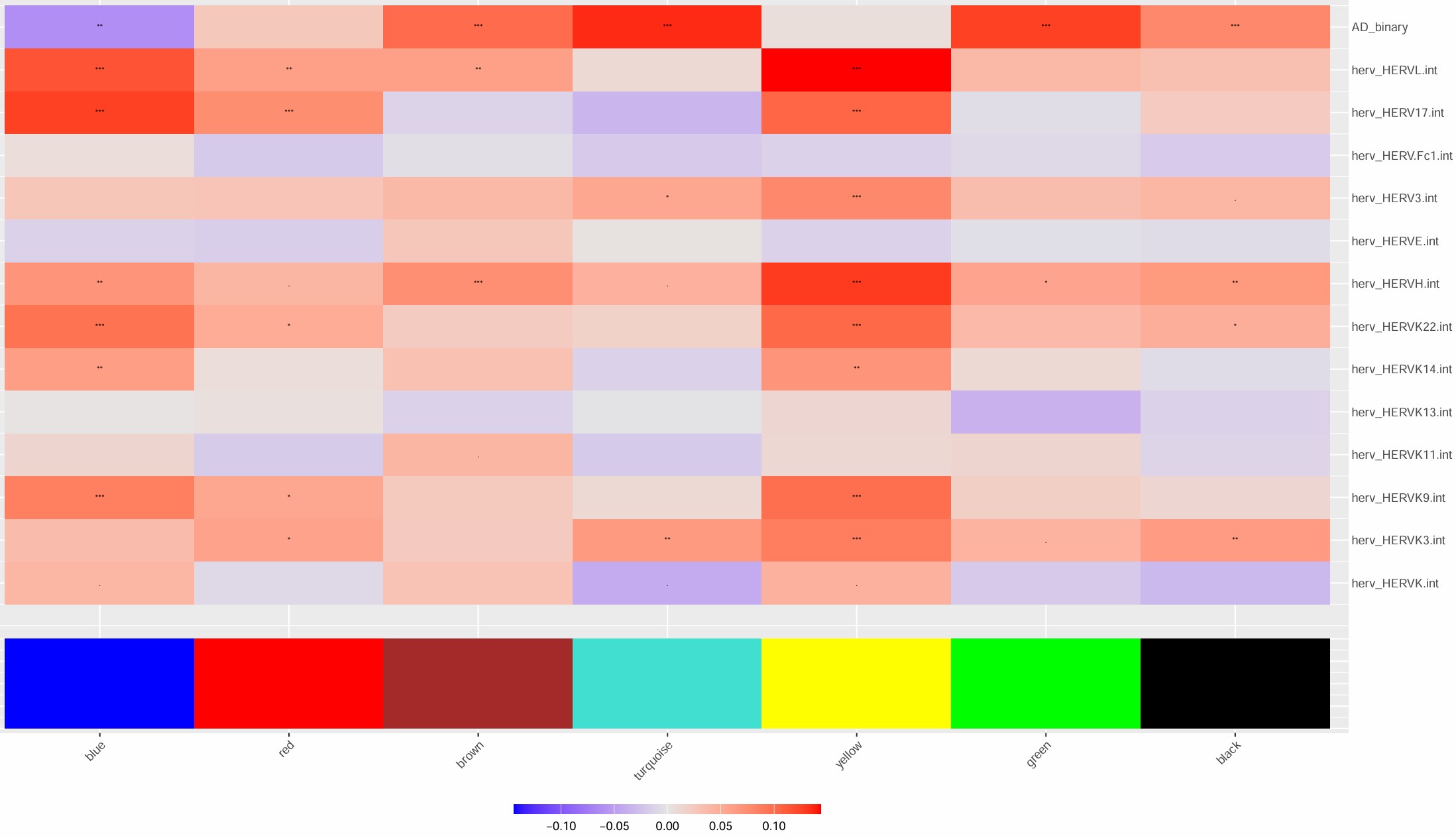
p <- PlotModuleTraitCorrelation(seu, label = "fdr", label_symbol = "stars")
print(p)
dev.off()
save(seu, file = file.path(res_dir, "oligo_WGCNA_try2.RData"))

     module n_genes
3      grey    3157
2 turquoise    1407
1      blue     201
5     brown      71
4    yellow      64
6     green      58
8       red      50
7     black      33
9      pink      21

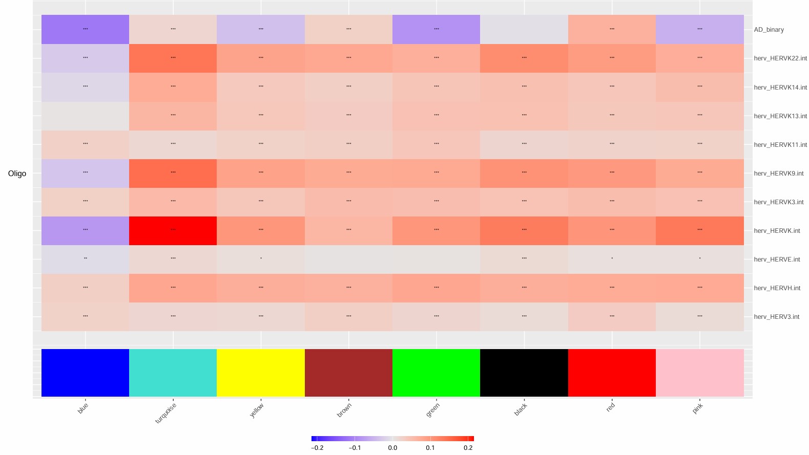
target_modules <- c("turquoise", "blue", "brown", "yellow", "green", "red")

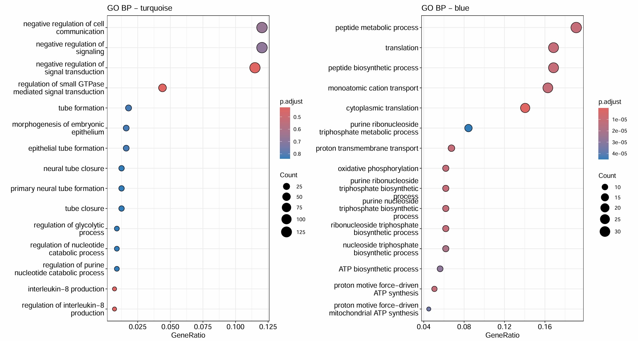
• turquoise和几乎所有hERV trait都是正相关，但基因数仍比较大（1400多个基因），GO结果里也有一些像small GTPase signaling/signal transduction negative regulation/actin cytoskeleton organization/IL-8 production这类看起来可能和AD有关的条目，但padj基本都不显著，属于广义状态程序
• blue的GO较集中且显著，都是关于能量代谢/蛋白合成的，hub genes也有不少核糖体/代谢相关基因：当hERV较高或AD状态更明显时，这套“翻译-氧化磷酸化-ATP合成”程序会下降
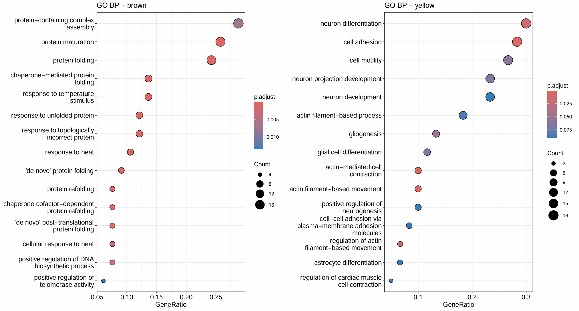
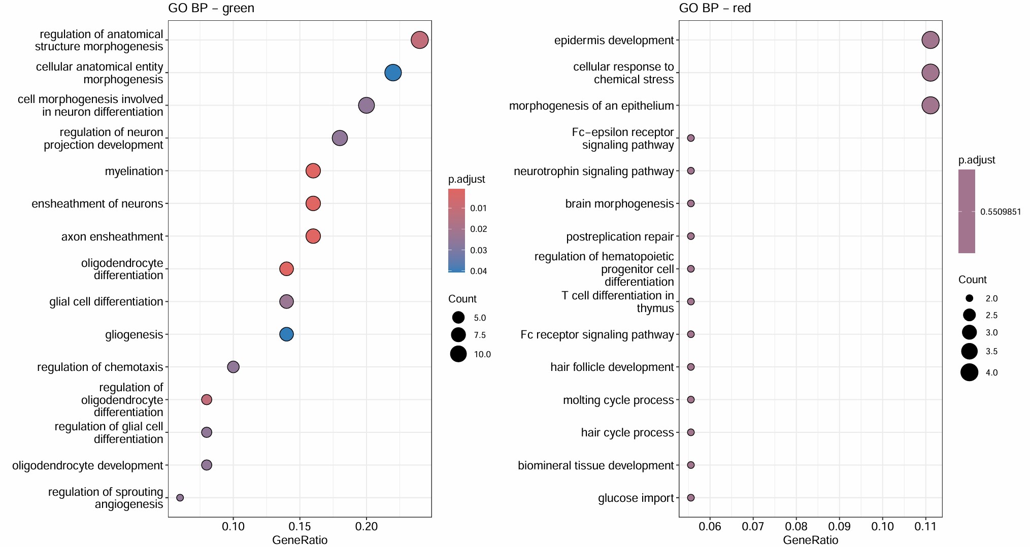
• green是少突分化/髓鞘形成模块，yellow是细胞黏附/神经突起/运动与分化模块，和hERVK都是正相关，和AD略偏负相关
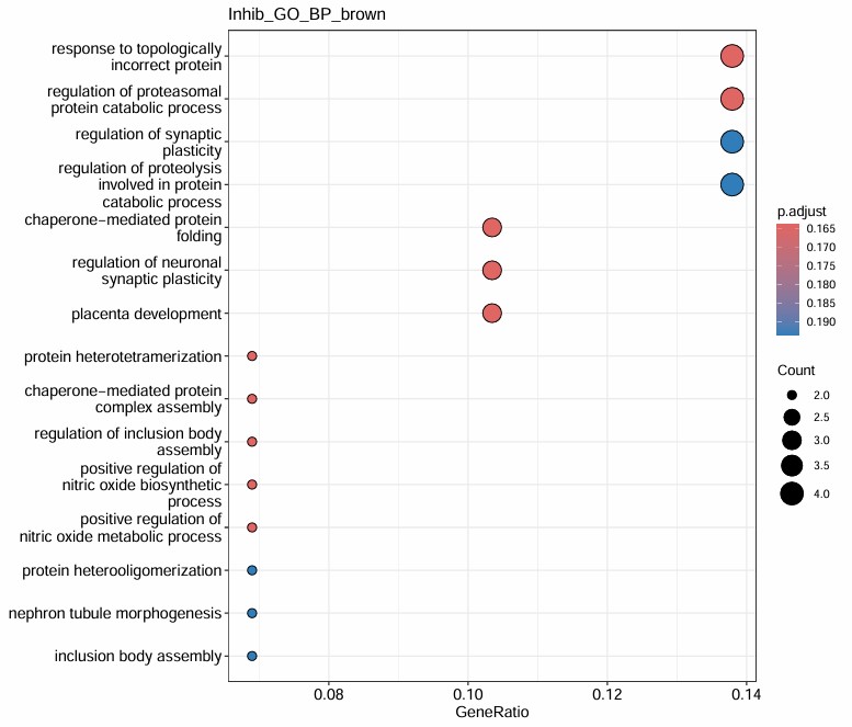
• brown是蛋白折叠/热休克/蛋白稳态模块，和AD/hERV都是轻度正相关，更像是一个病理相关的模块

---

亚群层面分析：

• 对于hERV高表达的亚群，分为AD富集/不富集两种，如果该亚群hERV高表达且AD多，就对应brown/turquoise/blue这类AD和hERV同步变化的基因模块（蛋白稳态/广义hERV激活状态/稳态代谢受损），如果AD少就更像green/yellow这种不同步变化的（少突成熟/髓鞘化/分化或形态重塑）
  • 理想情况是上面说的这样的，不过在我的亚群聚类时，至少在oligo的亚群里面，并没有出现某个亚群的AD特别富集，所以还是以模块表达分数为准
• 先看这个亚群的模块表达分数（就是上面得到的几个关键模块），看哪个模块在这个亚群里表达更高
• 把这个亚群和其它亚群做差异表达分析，得到一组亚群特异上调基因，看这些基因与各模块基因的重叠度，综合模块表达分数，确定这个亚群在哪个模块上特异表达
• 对DEG与目标模块内的基因取交集，再GO

load(file.path(res_dir, "oligo_WGCNA_try2.RData"))
seu_net <- seu
seu <- readRDS("/public/home/GENE_proc/wth/my_data/oligo.rds")
seu$subcluster <- seu$RNA_snn_res.0.5
wgcna_name <- "gene_net"
subcluster_col <- "subcluster"
target_clusters <- c("3", "5", "9")
modules_use <- c("brown", "turquoise", "blue", "green", "yellow")
# 取出模块基因
modules_df <- GetModules(seu_net, wgcna_name = wgcna_name)
gene_col <- intersect(c("gene_name", "gene", "feature"), colnames(modules_df))[1]
modules_df <- subset(modules_df, module %in% modules_use & module != "grey")
module_list <- split(modules_df[[gene_col]], modules_df$module)
module_list <- lapply(module_list, unique)
module_list <- lapply(module_list, intersect, rownames(seu[["RNA"]]))
# 给每个细胞打模块分数
for (m in modules_use) {
  seu <- AddModuleScore(
    seu,
    features = list(module_list[[m]]),
    assay = "RNA",
    name = paste0(m, "_score_")
  )
}
score_cols <- setNames(paste0(modules_use, "_score_1"), modules_use)
Idents(seu) <- seu[[subcluster_col]][, 1]
# 各亚群的模块平均分数
score_avg <- seu@meta.data[, c(subcluster_col, unname(score_cols)), drop = FALSE]
colnames(score_avg)[1] <- "subcluster"
score_avg <- score_avg %>%
  group_by(subcluster) %>%
  summarise(across(everything(), mean))
write.csv(score_avg, file.path(res_dir, "subcluster_module_scores.csv"), row.names = FALSE)
score_mat <- as.matrix(score_avg[, -1])
rownames(score_mat) <- score_avg$subcluster
colnames(score_mat) <- names(score_cols)
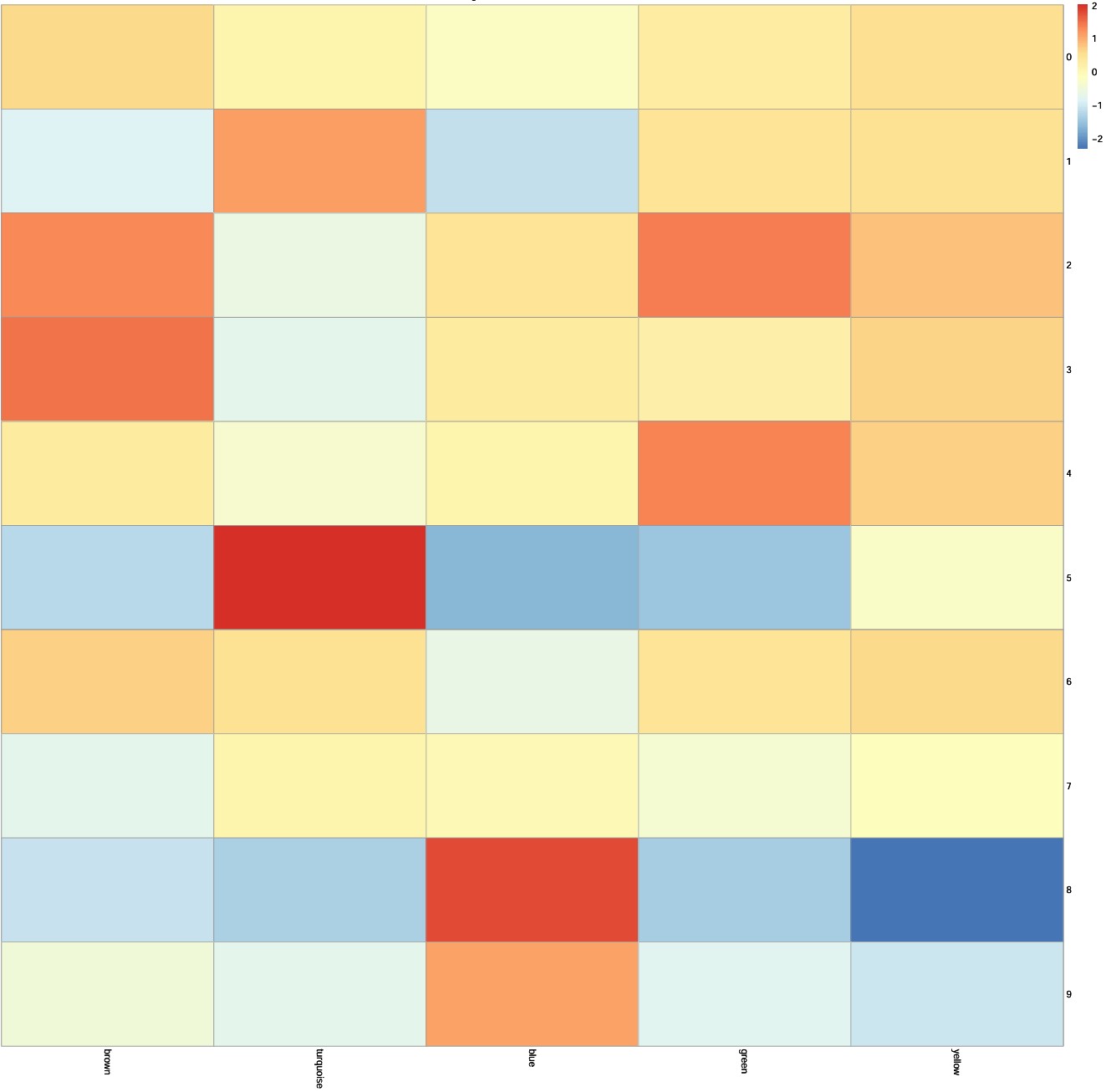
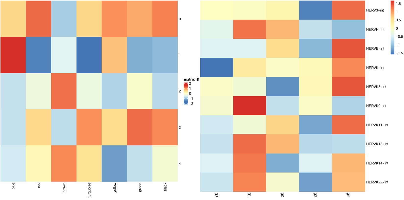
pdf(file.path(res_dir, "subcluster_module_scores.pdf"), width = 16, height = 16)
p <- pheatmap(
  scale(score_mat),
  cluster_rows = FALSE,
  cluster_cols = FALSE,
  main = "Scaled by module across subclusters"
)
print(p)
dev.off()

# 特异亚群与其它亚群的DEG
universe_genes <- unique(unlist(module_list))
Idents(seu) <- seu$subcluster
for (cl in target_clusters) {
  other_ids <- setdiff(levels(Idents(seu)), cl)
  deg <- FindMarkers(
    seu,
    ident.1 = cl,
    ident.2 = other_ids,
    assay = "RNA",
    slot = "data",
    test.use = "MAST",
    # latent.vars = c("nCount_RNA", "percent_mito"),
    min.pct = 0.1,
    logfc.threshold = 0
  )
  deg$gene <- rownames(deg)
  fc_col <- grep("^avg_log", colnames(deg), value = TRUE)[1]
  deg_up <- subset(deg, p_val_adj < 0.05 & deg[[fc_col]] > 0.1)
  write.csv(deg, file.path(res_dir, paste0("DEG_subcluster_", cl, "_all.csv")), row.names = FALSE)
  write.csv(deg_up, file.path(res_dir, paste0("DEG_subcluster_", cl, "_up.csv")), row.names = FALSE)
  target_mean <- colMeans(
    seu@meta.data[seu[[subcluster_col]][, 1] == cl, unname(score_cols), drop = FALSE]
  )
  other_mean <- colMeans(
    seu@meta.data[seu[[subcluster_col]][, 1] != cl, unname(score_cols), drop = FALSE]
  )
  score_tbl <- data.frame(
    module = names(score_cols),
    target_mean = unname(target_mean[unname(score_cols)]),
    other_mean  = unname(other_mean[unname(score_cols)]),
    stringsAsFactors = FALSE
  )
  score_tbl$score_diff <- score_tbl$target_mean - score_tbl$other_mean
  up_genes <- deg_up$gene
  overlap_tbl <- data.frame(
    module = names(score_cols),
    overlap_n = 0,
    gene_ratio = 0,
    fisher_p = 1,
    overlap_genes = "",
    stringsAsFactors = FALSE
  )
  for (m in names(score_cols)) {
    mod_genes <- module_list[[m]]
    hit_genes <- intersect(up_genes, mod_genes)
    a <- length(hit_genes)
    b <- length(setdiff(up_genes, mod_genes))
    c <- length(setdiff(mod_genes, up_genes))
    d <- length(setdiff(universe_genes, union(up_genes, mod_genes)))
    overlap_tbl[overlap_tbl$module == m, "overlap_n"] <- a
    overlap_tbl[overlap_tbl$module == m, "gene_ratio"] <- ifelse(length(up_genes) > 0, a / length(up_genes), 0)
    overlap_tbl[overlap_tbl$module == m, "overlap_genes"] <- paste(hit_genes, collapse = ";")
    overlap_tbl[overlap_tbl$module == m, "fisher_p"] <- fisher.test(
      matrix(c(a, b, c, d), nrow = 2),
      alternative = "greater"
    )$p.value
  }
  res_tbl <- left_join(score_tbl, overlap_tbl, by = "module") %>%
    arrange(desc(score_diff), fisher_p)
  write.csv(res_tbl, file.path(res_dir, paste0("subcluster_", cl, "_module_integration.csv")), row.names = FALSE)
}
save(module_list, universe_genes, file = file.path(res_dir, "0401.RData"))

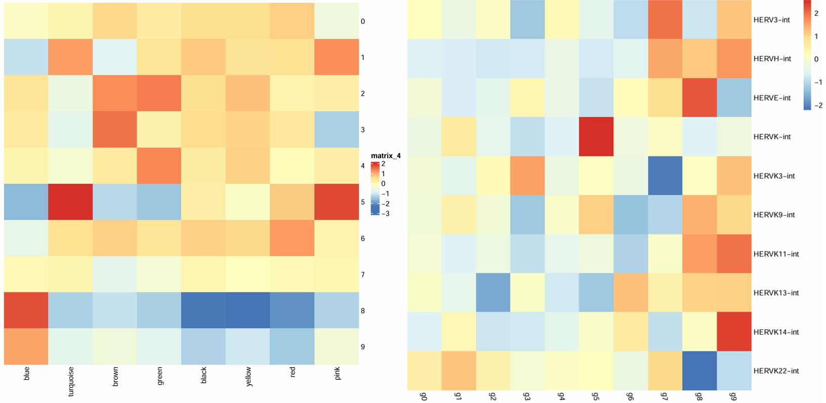
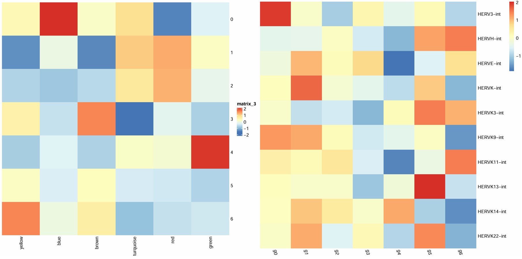
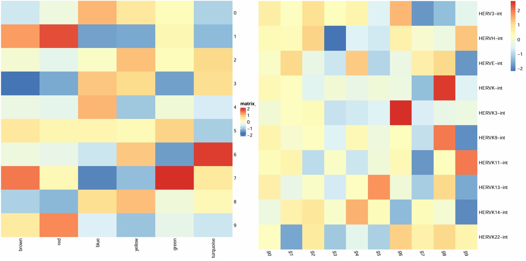
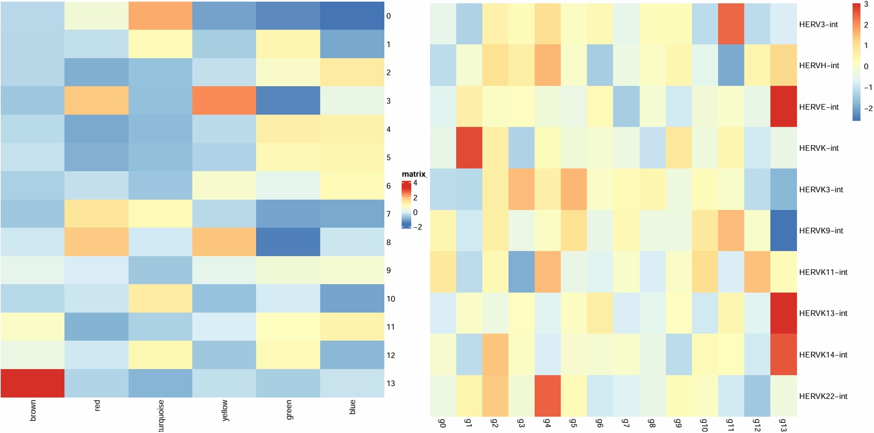
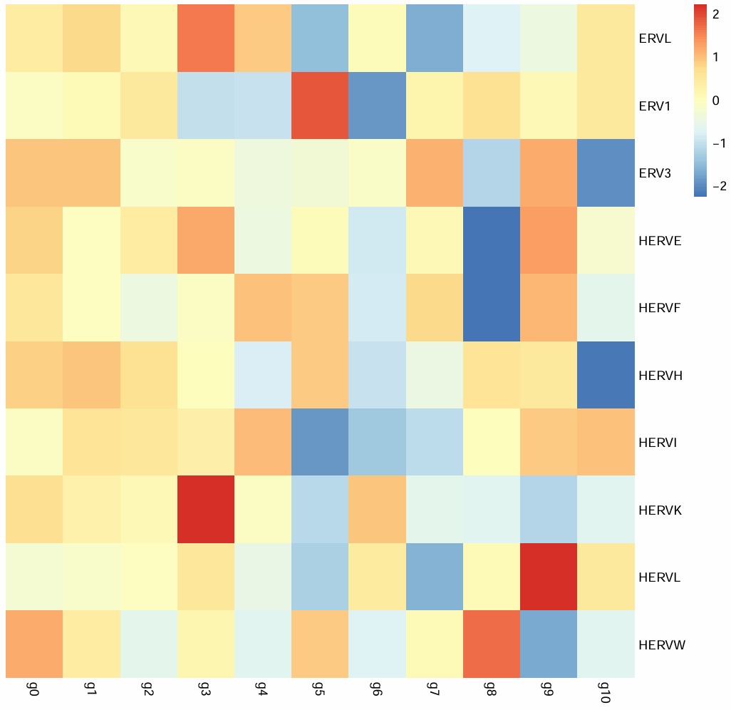
之前做的oligo各cluster的hERV平均表达量热图：

cluster 5：

• 从表达量热图中可以看到它的hERVK/hERVK9比较高
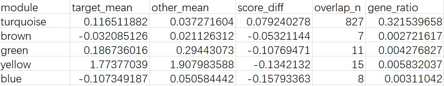
• turquoise score_diff比较高，且上调DEG与turquoise的重叠较多
• 最像广义hERV激活状态

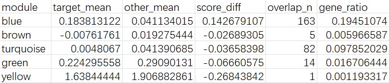
cluster 3：

• HERVK3比较高
• 上调基因包括ARHGAP24/CTNNA2/PTPRM/DCC/BCAN/ITPR2/PLEKHH2，属于细胞黏附/细胞骨架/发育的模块，与yellow模块的GO结果吻合
• 像结构重塑/形态变化/分化相关亚群

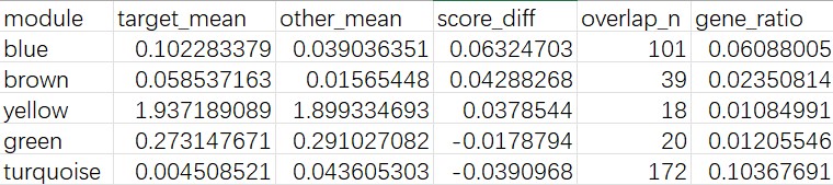
cluster 9：

• HERVK家族普遍较高
• 虽然上调基因有一些偏向神经元的标记基因，不过画了一下dotplot发现整体上更偏向oligo而不是神经元
• blue模块分数较高

target_module_map <- c(
  "5" = "turquoise",
  "3" = "yellow",
  "9" = "blue"
)
plot_list <- list()
for (cl in names(target_module_map)) {
  deg_up <- read.csv(
    paste0("C:\\Users\\17185\\Desktop\\fsdownload\\DEG_subcluster_", cl, "_up.csv"),
    stringsAsFactors = FALSE
  )
  target_module <- target_module_map[[cl]]
  gene_use <- intersect(deg_up$gene, module_list[[target_module]])
  write.csv(
    data.frame(gene = gene_use),
    paste0("C:\\Users\\17185\\Desktop\\fsdownload\\subcluster_", cl, "_", target_module, "_intersect_genes.csv"),
    row.names = FALSE
  )
  ego <- enrichGO(
    gene = gene_use,
    universe = universe_genes,
    OrgDb = org.Hs.eg.db,
    keyType = "SYMBOL",
    ont = "BP",
    pAdjustMethod = "BH",
    pvalueCutoff = 1,
    qvalueCutoff = 1,
    readable = TRUE
  )
  ego_df <- as.data.frame(ego)
  write.csv(
    ego_df,
    paste0("C:\\Users\\17185\\Desktop\\fsdownload\\subcluster_", cl, "_", target_module, "_GO_BP.csv"),
    row.names = FALSE
  )
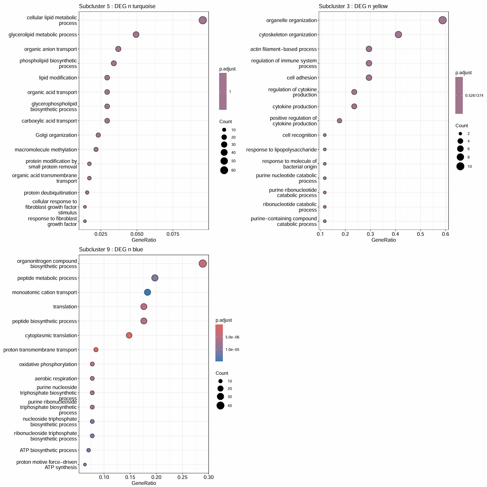
  plot_list[[cl]] <- dotplot(ego, showCategory = 15) +
    ggtitle(paste0("Subcluster ", cl, " : DEG ∩ ", target_module))
}
pdf(file.path(res_dir, "oligo_359_GO_summary.pdf"), width = 16, height = 16)
p <- wrap_plots(plot_list, ncol = 2)
print(p)
dev.off()

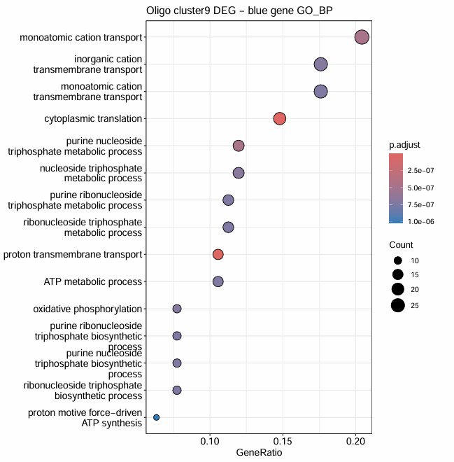
• cluster 9的GO结果是唯一真正显著的，且GO富集条目与blue亚群吻合，说明它最可能代表的是：一个翻译活跃、线粒体呼吸活跃、能量代谢强、同时又保留成熟髓鞘marker的少突亚群

  结合前面的hERV表达量热图，可以理解成：cluster 9虽然也是hERV-high，但它对应的不是 “HERVK-int驱动的广义激活状态”，而更像一种“成熟髓鞘化背景下的hERV表达模式”

• cluster 5的GO结果虽然不显著，但也符合turquoise模块的GO结果，在功能上呈现出脂质代谢、膜转运、去泛素化和FGF反应等倾向。说明交集基因虽然多，但功能比较分散

  它是最像hERV激活型的亚群，只是它的功能解释更适合写成脂质与膜代谢重塑、广义信号调节

• cluster 3的GO结果与5类似，它确实更偏向细胞骨架/黏附/actin重塑/与外界刺激或炎症反应有关的调节，像是一个结构重塑/黏附变化/分化过程中的亚群

总结：hERV高表达在少突细胞内并不对应单一病理程序，而是和不同的细胞状态相联系

• cluster 5：hERVK/K9主导的广义激活型

  功能倾向：脂质代谢、膜转运、信号/修饰重塑

• cluster 3：HERVK3相关的结构重塑型

  功能倾向：actin、黏附、形态/细胞识别

• cluster 9：多种hERV相关的成熟髓鞘化/高代谢型

  功能：翻译、氧化磷酸化、ATP合成

方案2

mixed_herv_features <- c("HERV3-int", "HERVH-int", "HERVE-int", "HERVK-int", "HERVK3-int", "HERVK9-int", "HERVK11-int", "HERVK13-int", "HERVK14-int", "HERVK22-int")
# 过滤掉表达比例<5%的基因（为防止把加进去的hERV也过滤掉，所以就不在SetupForWGCNA时过滤）
rna_counts <- LayerData(seu, assay = "RNA", layer = "counts")
feature_rowsum <- Matrix::rowSums(rna_counts > 0)
retained_f_low <- feature_rowsum > ncol(seu) * 0.05
genes_keep <- names(feature_rowsum)[retained_f_low]
seu[["RNA"]] <- subset(seu[["RNA"]], features = genes_keep)
# 构建混合assay：RNA gene + hERV feature
rna_counts <- LayerData(seu, assay = "RNA", layer = "counts")
rna_data  <- LayerData(seu, assay = "RNA", layer = "data")
herv_counts <- LayerData(seu, assay = herv_assay, layer = "counts")[mixed_herv_features, , drop = FALSE]
herv_data <- LayerData(seu, assay = herv_assay, layer = "data")[mixed_herv_features, , drop = FALSE]
rownames(herv_counts) <- paste0("HERV__", rownames(herv_counts))
rownames(herv_data) <- paste0("HERV__", rownames(herv_data))
mixed_counts <- rbind(rna_counts, herv_counts)
mixed_data <- rbind(rna_data, herv_data)
seu[["RNA_HERV"]] <- CreateAssayObject(counts = mixed_counts)
LayerData(seu, assay = "RNA_HERV", layer = "data") <- mixed_data
DefaultAssay(seu) <- "RNA_HERV"
mixed_features <- rownames(seu[["RNA_HERV"]])
# 重复前述步骤
seu <- SetupForWGCNA(
  seu,
  gene_select = "custom",
  gene_list = mixed_features,
  assay = "RNA_HERV",
  wgcna_name = "mixed_net"
)
seu <- MetacellsByGroups(
  seurat_obj = seu,
  group.by = c("celltype", "orig.ident"),
  ident.group = "celltype",
  assay = "RNA_HERV",
  layer = "data",
  reduction = "pca",
  dims = 1:30,
  k = 25,
  max_shared = 10,
  min_cells = 50,
  mode = "average",
  wgcna_name = "mixed_net"
)
seu <- NormalizeMetacells(seu, wgcna_name = "mixed_net")
seu <- SetDatExpr(
  seu,
  group_name = celltype_name,
  group.by = "celltype",
  use_metacells = TRUE,
  assay = "RNA_HERV",
  layer = "data",
  wgcna_name = "mixed_net"
)
grep("^HERV__", rownames(seu))
seu <- TestSoftPowers(
  seu,
  networkType = "signed",
  wgcna_name = "mixed_net"
)
power_table_mixed <- GetPowerTable(seu)
soft_power_mixed <- power_table_mixed$Power[which(power_table_mixed$SFT.R.sq >= 0.8)[1]]
if (is.na(soft_power_mixed)) {
  soft_power_mixed <- power_table_mixed$Power[which.max(power_table_mixed$SFT.R.sq)]
}
plot_list <- PlotSoftPowers(seu)
pdf(file.path(res_dir, "oligo_soft_power2.pdf"), width = 16, height = 16)
p <- patchwork::wrap_plots(plot_list, ncol = 2)
print(p)
dev.off()
save(seu, file = file.path(res_dir, "oligo_WGCNA2_before_ConstructNetwork.RData"))
seu <- ConstructNetwork(
  seu,
  assay = "RNA_HERV",
  soft_power = soft_power_mixed,
  networkType = "signed",
  tom_name = "seu_TOM",
  overwrite_tom = TRUE,
  wgcna_name = "mixed_net"
)
seu <- ScaleData(
  seu,
  assay = "RNA_HERV",
  features = rownames(seu[["RNA_HERV"]]),
)
seu <- ModuleEigengenes(
  seu,
  # group.by.vars = "orig.ident",
  assay = "RNA_HERV",
  wgcna_name = "mixed_net"
)
seu <- ModuleConnectivity(
  seu,
  group.by = "celltype",
  group_name = celltype_name,
  assay = "RNA_HERV",
  wgcna_name = "mixed_net"
)
save(seu, file = file.path(res_dir, "oligo_WGCNA2.RData"))

module_genes_df <- GetModules(seu)
hub_genes_df <- GetHubGenes(seu, n_hubs = 50)
modules <- unique(module_genes_df$module)
genes_list <- list()
for(single_module in modules){
  module_genes <- module_genes_df %>%
    filter(module == single_module) %>%
    pull(gene_name) %>%
    unique()
  genes_list[[single_module]]$module_genes <- module_genes
  hub_genes <- hub_genes_df %>%
    filter(module == single_module) %>%
    pull(gene_name) %>%
    unique()
  genes_list[[single_module]]$hub_genes <- hub_genes
}
TOM <- GetTOM(seu)
target_herv <- grepl("^HERV--", colnames(TOM))  # 目标hERV
target_gene <- !grepl("^HERV--", rownames(TOM))  # gene
universe_genes <- rownames(TOM)[target_gene]
herv_neighbors <- as.data.frame(TOM[target_gene, target_herv]) %>% 
  rownames_to_column("rowname") %>% 
  as_tibble() %>%
  column_to_rownames("rowname")
res_list <- list()
for(herv in colnames(herv_neighbors)){
  herv_gene <- herv_neighbors[, herv, drop = FALSE]
  colnames(herv_gene) <- "value"
  herv_module <- subset(module_genes_df, gene_name == herv)$module
  print(paste0(herv, "所属的模块为：", herv_module))
  module_genes <- subset(module_genes_df, module == herv_module)$gene_name
  res_list[[herv]]$module <- herv_module
  cor_gene <- subset(herv_gene, rownames(herv_gene) %in% module_genes) %>%
    filter(abs(value) > 0.02) %>%
    arrange(desc(value)) %>%
    head(n = 300) %>%
    rownames_to_column("gene")
  res_list[[herv]]$cor <- cor_gene
  res_list[[herv]]$cor_range <- c(max(cor_gene$value), min(cor_gene$value))
  res_list[[herv]]$gene <- cor_gene$gene
}
save(genes_list, res_list, universe_genes, file = file.path(res_dir, "oligo_WGCNA2_res.RData"))

"HERV--HERV3-int所属的模块为：grey"
"HERV--HERVH-int所属的模块为：blue"
"HERV--HERVE-int所属的模块为：grey"
"HERV--HERVK-int所属的模块为：turquoise"
"HERV--HERVK3-int所属的模块为：grey"
"HERV--HERVK9-int所属的模块为：turquoise"
"HERV--HERVK11-int所属的模块为：blue"
"HERV--HERVK13-int所属的模块为：grey"
"HERV--HERVK14-int所属的模块为：grey"
"HERV--HERVK22-int所属的模块为：turquoise"

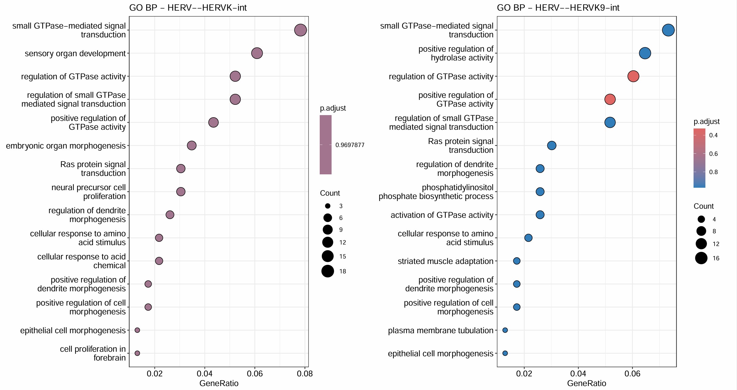
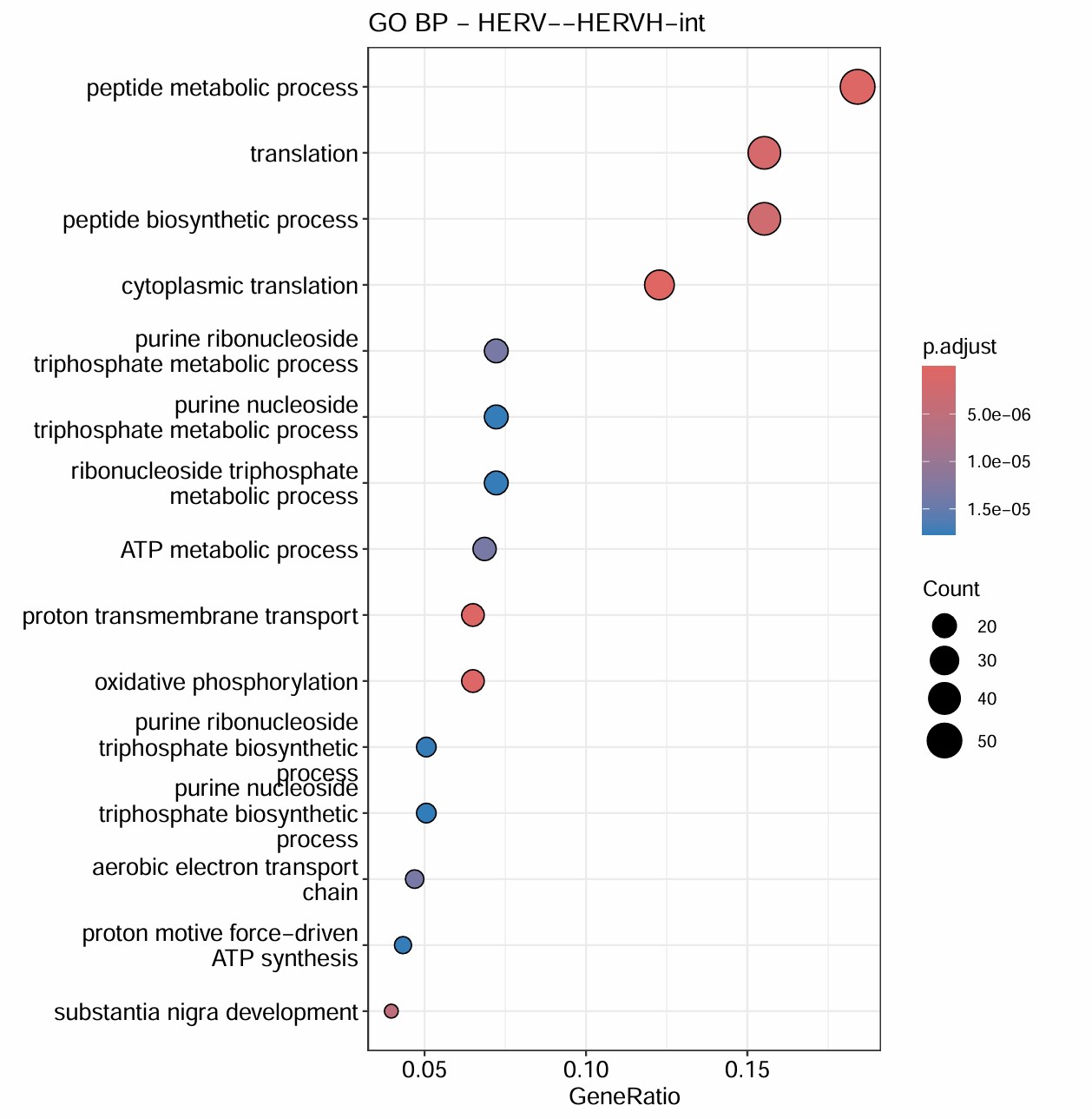
GO富集分析：

• 对HERVK/HERVK9/HERVK22/HERVH/HERVK11这几个不在grey模块（grey模块就是指比较模糊/没法聚类的基因）里的hERV相关性前300的基因做GO
• 对它们所在的模块做GO

# 前300基因
target_hervs <- c("HERV--HERVK-int", "HERV--HERVK9-int", "HERV--HERVK22-int", "HERV--HERVK11-int", "HERV--HERVH-int")
go_list <- lapply(target_hervs, function(m) {
  run_go_one(
    gene_vec = res_list[[m]]$gene,
    universe_genes = universe_genes,
    ont = "BP"
  )
})
names(go_list) <- target_hervs
res <- list()
for (m in target_hervs) {
  ego <- go_list[[m]]
  if (is.null(ego)) next
  res[[m]] <- dotplot(ego, showCategory = 15) +
    ggtitle(paste0("GO BP - ", m))
}
pdf(file.path(res_dir, "oligo_hERV_gene_summary.pdf"), width = 15, height = 24)
p <- wrap_plots(res, ncol = 2)
print(p)
dev.off()
oligo_hERV_gene_summary <- lapply(target_hervs, function(m) {
  ego <- go_list[[m]]
  if (is.null(ego)) return(NULL)
  go_df <- as.data.frame(ego)
  go_df <- go_df[order(go_df$p.adjust), ]
  herv_list <- res_list[[m]]
  data.frame(
    herv = m,
    module = as.character(herv_list$module),
    cor_gene = paste(herv_list$gene, collapse = "; "),
    max_cor = herv_list$cor_range[1],
    min_cor = herv_list$cor_range[2],
    GO = paste(go_df$Description[1:20], collapse = "; "),
    GO_padj = paste(go_df$p.adjust[1:20], collapse = "; "),
    stringsAsFactors = FALSE
  )
}) %>% bind_rows()
write.csv(oligo_hERV_gene_summary, file.path(res_dir, "oligo_hERV_gene_summary.csv"), row.names = FALSE)

# 它们所在的模块
target_modules <- unique(as.character(oligo_hERV_gene_summary$module))
go_list <- lapply(target_modules, function(m) {
  run_go_one(
    gene_vec = genes_list[[m]]$module_genes,
    universe_genes = universe_genes,
    ont = "BP"
  )
})
names(go_list) <- target_modules
res <- list()
for (m in target_modules) {
  ego <- go_list[[m]]
  if (is.null(ego)) next
  res[[m]] <- dotplot(ego, showCategory = 15) +
    ggtitle(paste0("GO BP - ", m))
}
pdf(file.path(res_dir, "oligo_hERV_module_summary.pdf"), width = 16, height = 8)
p <- wrap_plots(res, ncol = 2)
print(p)
dev.off()
oligo_hERV_module_summary <- lapply(target_modules, function(m) {
  ego <- go_list[[m]]
  if (is.null(ego)) return(NULL)
  go_df <- as.data.frame(ego)
  go_df <- go_df[order(go_df$p.adjust), ]
  module_list <- genes_list[[m]]
  data.frame(
    module = m,
    n_gene = length(module_list$module_genes),
    hub_gene = paste(module_list$hub_genes, collapse = "; "),
    GO = paste(go_df$Description[1:20], collapse = "; "),
    GO_padj = paste(go_df$p.adjust[1:20], collapse = "; "),
    stringsAsFactors = FALSE
  )
}) %>% bind_rows()
write.csv(oligo_hERV_module_summary, file.path(res_dir, "oligo_hERV_module_summary.csv"), row.names = FALSE)

综合上面的结果，HERVH-int和HERVK11-int的GO结果最显著，且它们都在blue这个module，对该模块的GO分析结果也显著集中于蛋白翻译+线粒体能量代谢。另外几个都在turquoise模块，不过这个模块的GO结果与方案1的类似，都比较模糊

• 一个比较大的问题就是与hERV相关的前300个基因的相关性在0.05±0.02左右，这个相关性应如何衡量？

  这个相关性实际上不是前面线性拟合时得到的相关性，而是TOM相似度，这种计算方法得到的数值会比普通相关系数小很多，因此这个值其实不能说是“弱相关”

接下来的GO分析与上面方案1的类似，都是计算目标亚群与其它亚群的DEG，然后看目标亚群的高表达hERV相邻的基因与DEG的重叠度，取两者重合的部分作GO

共表达网络

选hERV特异亚群和显著神经相关模块进行GO分析

以下结果，如果family和group的没有太大差别，就只展示family的结果，后期也以family为主进行分析

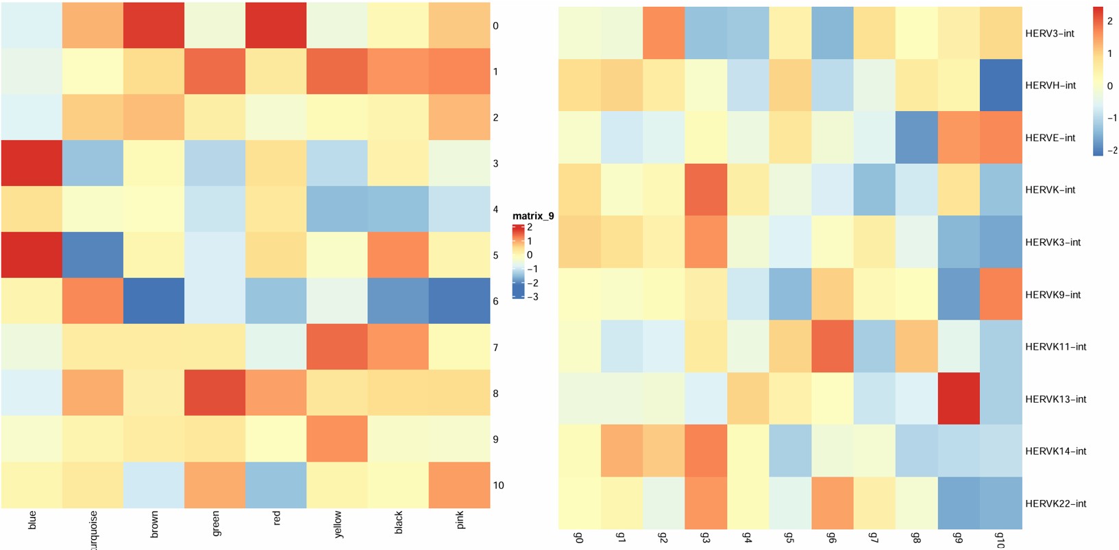
hERV表达量热图是按行看——每个hERV家族在各亚群中的相对表达水平，模块分数热图是按列看，每个模块在各亚群中的相对表达水平（其实只是行列倒过来了，意义相同）

Oligo

汇总一下之前的记录：

Astro

• 0在blue表达量高，blue和hERVK有正相关，和AD微弱负相关，可作为目标亚群
• 1在red表达量高，但red和hERV相关性较弱，不如0+blue

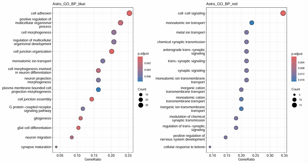
• blue和red都有神经相关的条目，其中blue神经相关条目看起来非常多

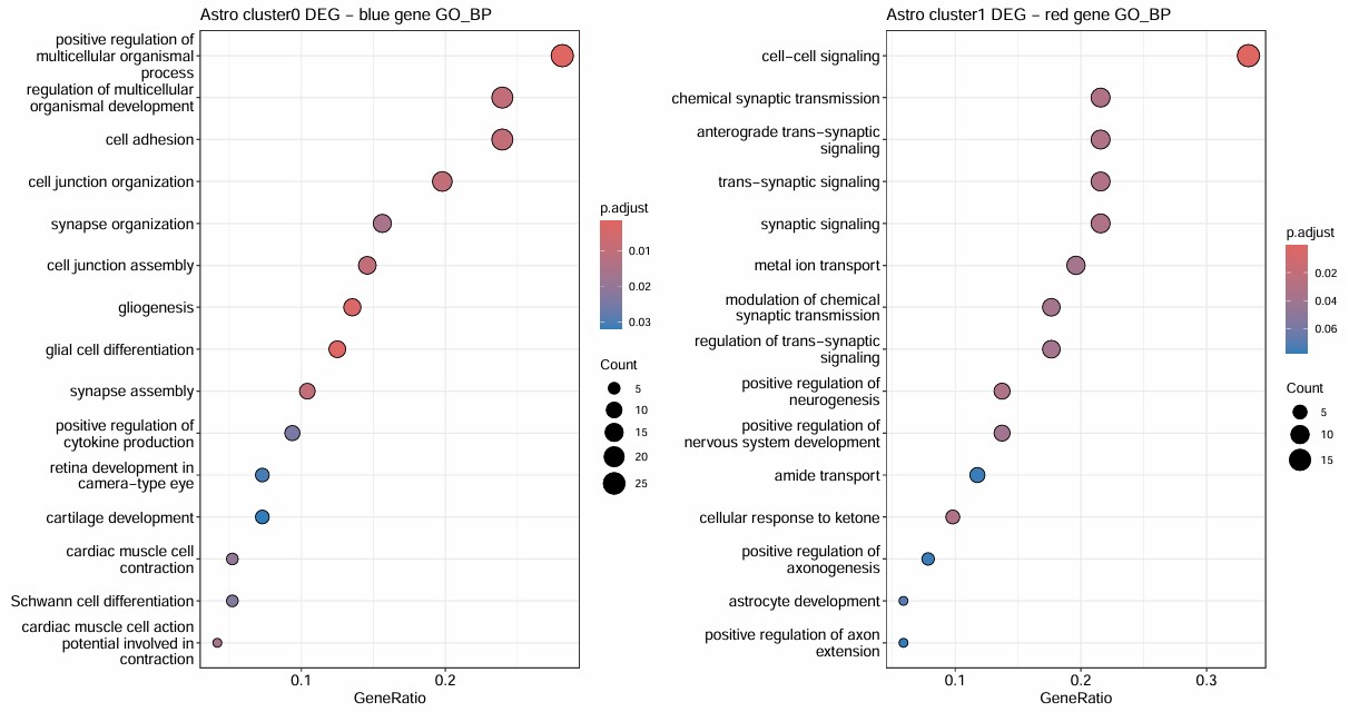
• cluster0有15000个细胞，占astro的3/4，AD占比很平均
• cluster1有3000多个细胞，AD稍微多一些（比astro整体AD占比多3%）
• 但是它们的GO聚类结果很好，blue和神经功能显著相关，red也较显著，和信号传导相关

OPC

• 6在turquoise表达量高，turquoise和hERVK有正相关，和AD无相关，可作为目标亚群
• 8没有特别高的，只有yellow有点点高，但yellow和hERV相关性不如6+turquoise

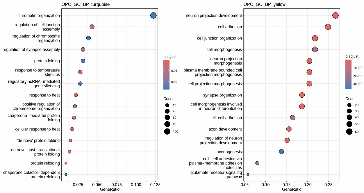
• yellow和astro的blue几乎一模一样，turquoise更偏普通功能，也有染色体结构/转录翻译这些
• 然而不知道为什么OPC的6/8亚群的DEG只有十几个，取交集后就只剩下个位数了

Excit

• 6hERV下调，在blue/green/magenta/pink模块也下调，在black/red/yellow模块上调
  • blue/green/magenta/pink与hERV都正相关
  • black与hERV负相关程度很大，red其次，yellow相关程度较低
  • 因此可以看看6与blue/green/magenta/pink/black/red这几个模块

• 每个模块都有一些看起来和神经/免疫相关的，但都不太显著
  • black和red和神经比较相关
  • pink和免疫有关
  • green和DNA/RNA有关
• 考虑到6在black和red下调，所以应该取6亚群下调基因与它们的交集

• 6有近3000个细胞，NC略多（1.4%），但其上调基因确实显著富集到神经相关条目上，black和pink模块与hERV负相关，6在这两个模块上调，且hERV表达量低

Inhib

• 2没有特别负相关的模块，不过brown与hERV负相关，且2在其中表达很低，可以看看2和brown的关系

• 感觉没什么特别的

Endo

• 1在blue上调，red/turquoise下调
• 4在brown上调，yellow下调
• 主线应该就是1和blue，yellow相关性不太稳定

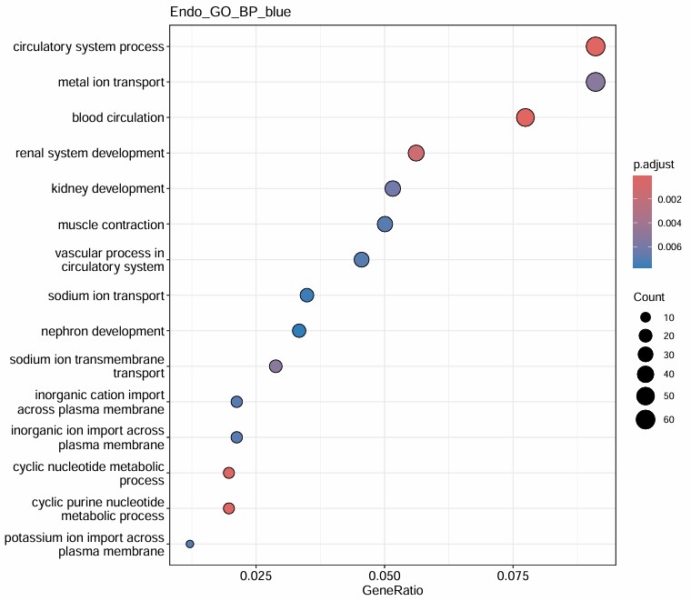
• blue基因数似乎太多了，感觉也没什么特别的

Mic

• blue和hERV显著负相关，3hERV表达高，但blue模块表达量也高，这对吗？
• 6在turquoise上调，brown/pink/black/red下调，然而turquoise/brown/pink/black/red都和hERV正相关，最主要6就100多个细胞，不太行
• 只有2有1000多个细胞，在blue微微下调，在turquoise/brown/pink微上调
• 如果mic很值得一看的话，大概就是blue/turquoise/brown/pink

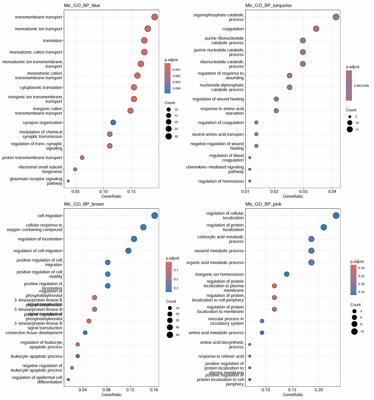
• blue的结构比较显著，与神经和翻译有相关，其它几个感觉有点普通了，可以先做个取交集看看
• 考虑到2在blue下调，所以应该取2亚群下调基因与它的交集

• 2AD多（13%），在blue这个神经相关模块下调，且hERVK等家族表达量高，hERVK与blue显著负相关；在pink这个信号响应？模块上调，pink与hERV正相关

• 补一下mic的group热图，与hERVK的关系看得更明显

  

所有亚群的GO分析

对所有模块进行一遍GO分析，看有没有免疫相关模块、炎症相关模块(Mic)，补充一下之前的结论

astro：也存在免疫/细胞因子响应方向的hERV关联，但强度和清晰度不如Mic，更像是“胶质支持/分化+轻度炎症响应”的背景状态

• blue：与hERV明显正相关，更偏向一个胶质分化/细胞黏附/神经支持相关状态
• green：与hERV也有正相关，TNF/cytokine response
• yellow：显著富集到蛋白质相关条目，与hERV有弱相关
• turquoise：与DNA修复有关，与hERV强正相关，但GO不显著

Oligo：hERV更稳定地关联到一个“广义信号调节/状态重塑”模块；但在具体亚群层面，某些hERV-high状态（比如cluster 9）又可以进一步落到“高翻译/高代谢/成熟髓鞘化”程序上

• turquoise和hERV相关性最强，GO条目分布比较广（该亚群基因数很多）
• green：成熟少突/髓鞘化模块，和hERV相关性一般
• brown：蛋白折叠/伴侣蛋白模块，和hERV相关性一般

Mic：hERV高表达更倾向于和先天免疫/炎症样程序增强相联系，同时与翻译/神经互作样程序下降相联系

• black：最像“先天免疫/抗病原体”模块，与hERV相关性较高
• pink：最像“炎症受体/信号响应”模块，虽然GO条目不是很集中，但hub gene中有TLR2/SP100/MAP3K8/EPSTI1，与炎症刺激/先天免疫信号响应有关
• yellow：蛋白折叠+免疫效应，可能说明Mic的hERV-high状态，可能不是单纯炎症，也可能伴随proteostasis/stress response
• blue：有cytoplasmic translation/synaptic signaling/glutamate receptor signaling/ribosome biogenesis条目，与hERV是负相关，可能说明Mic的hERV升高并不是简单伴随“全局活性增强”，而更像伴随某种homeostatic/neuron-interacting/translation-high状态的下降

Excit：hERV还可能与核酸代谢/复制样异常程序相关

• green模块的GO条目与DNA复制/核酸加工/应激样有关，且与hERV相关性较强，但GO不显著，也不是很标准的表观染色质调控模块

Inhib：与hERV相关性整体较弱，turquoise模块与hERV相关性较强，模块显著富集到突触相关条目，且与AD有弱负相关；brown与hERV有较强负相关，与蛋白折叠/应激有关，但GO不显著，可作为补充说明

Endo：与hERV相关性整体较弱，不过也有涉及到DNA合成/细胞分裂的yellow模块与hERV相关性较强，但GO不显著；brown显著富集到神经相关条目、green显著富集到蛋白质相关条目，但它们与hERV相关性较弱

有没有“STAT1等抗病毒通路相关的hERV”：

• STAT1指的是标准抗病毒程序：细胞感受到病毒核酸/dsRNA，从而激活免疫通路（type I / type II interferon）
• 上面提到的先天免疫/炎症样/抗原呈递样模块：细胞感受到损伤、病原相关分子、细胞碎片、炎症因子，通过TLR/NF-κB/MAPK/cytokine等通路进入激活状态，同时可能伴随吞噬、补体、抗原呈递等功能增强
• Mic中没有看到一个很典型的“STAT1-IFIT-OAS-MX1”式干扰素模块，有defense response/innate immune/TLR2/EPSTI1/MAP3K8（先天免疫/炎症样和抗原呈递样模块），不算特别像标准interferon/STAT1 signature
• OPC的green模块的hub gene里有STAT1，GO也有response to external biotic stimulus/response to other organism，与hERV也是正相关，但GO富集并不显著

总结byGPT

hERV关联不是统一的，而是明显细胞类型依赖：

• Astro、Oligo、OPC、Excit的模块-hERV相关性幅度更大
• Mic相关性中等，但模块的生物学解释很有意思
• Endo、Inhib整体较弱

AD和hERV不是简单同向：

• 很多模块里都能看到hERV和模块相关明显，但AD_binary相关很弱，甚至方向相反
• hERV更像是“细胞状态轴”的标志，而不是简单的AD/NC二分类标志

主线：

• Oligo：在整体层面，hERV更稳定地关联到“广义信号调节/状态重塑”模块。但在具体亚群层面，hERV高表达并不对应单一转录程序，而是分化为至少三类状态——一类偏膜脂与信号重塑，一类偏细胞骨架/黏附重塑，另一类则表现为成熟髓鞘化背景下的高翻译和高氧化磷酸化状态
  • cluster 5：更像hERV激活型，偏脂质代谢、膜转运、信号/修饰重塑
  • cluster 3：更像结构重塑/黏附变化/分化相关状态
  • cluster 9：最清楚，GO直接落在cytoplasmic translation/oxidative phosphorylation/ATP metabolic process，这说明它是一个成熟髓鞘化、高代谢、高翻译活性的少突状态
• Mic：在整体层面，hERV高表达状态与抗病毒/先天免疫样反应增强相关，同时伴随翻译/神经互作相关程序的下降
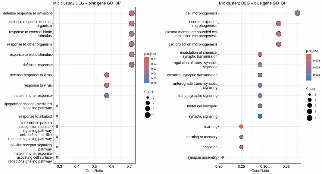
  • cluster 2：AD偏多（比全部Mic中的AD比例多13%），hERVK等家族偏高，与hERV正相关的pink模块上调，而pink模块富集到defense response to virus/response to virus/defense response to symbiont相关（DEG包括TLR2/MX2/MX1）；与hERV负相关的blue模块下调，blue模块与learning/cognition/trans-synaptic signaling/neuron projection morphogenesis相关
  • 除了pink和blue模块，在整体层面，Mic中的hERV与有关先天免疫/抗病原体的black模块、有关蛋白折叠和免疫效应的yellow模块有相关

支持性结果：

• Excit：提供了一个和神经胶质细胞不同的模式——是hERV较低的神经元状态，保留了更强的突触传递和囊泡循环程序；反过来说，hERV更多和激活/重塑/炎症类状态一起出现，hERV升高可能与神经元突触功能程序的减弱相关
  • cluster 6的hERV表达量低，在red和black模块上调，而red和black的GO都是突触和信号传递相关的
• astro：hERV相关模块主要连接到gliogenesis、cell-cell signaling和synapse organization，提示其更可能反映胶质细胞参与神经支持和细胞间通讯的状态，也存在免疫/细胞因子响应方向的hERV关联，但强度和清晰度不如Mic，更像“胶质支持/分化+轻度炎症响应”的背景状态

总述：hERV重调在AD脑内具有明显的细胞类型和细胞状态依赖性。在不同细胞类型中，hERV并非统一对应同一种病理程序，而是分别耦联到不同的转录模块：在oligo中与膜脂重塑、细胞骨架重塑及成熟髓鞘化/高代谢状态相关；在mic中与广义先天免疫/炎症样激活、抗原呈递样程序增强相关，并与稳态和翻译程序下降相关；在astro中更多关联于胶质分化、神经支持与轻度细胞因子响应；而在excit中，hERV升高则更可能与突触传递程序减弱相联系。除此之外，在OPC中也存在一定STAT1/外源刺激响应线索，在inhib中与突触功能和蛋白折叠/应激有关，在endo中与DNA合成/细胞分裂、神经和蛋白质相关功能有关，但与hERV的相关性较弱或者是GO富集结果不显著，需要更多验证

Figure1&S1

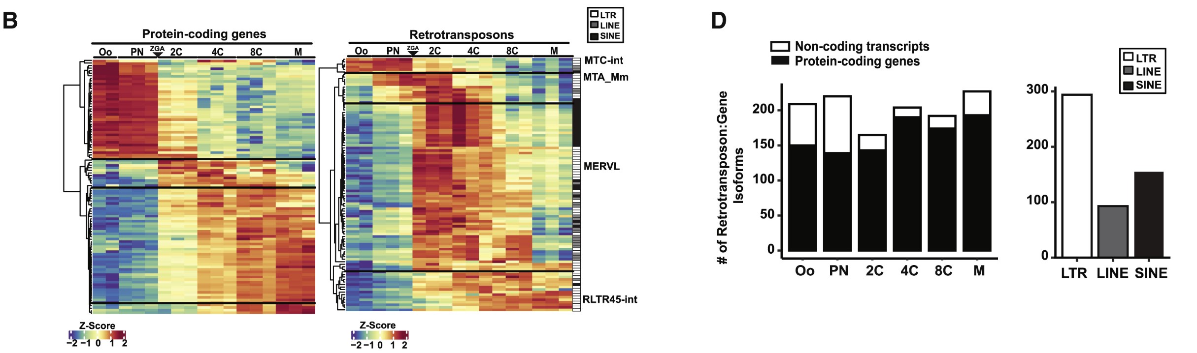
• 1B：在小鼠胚胎发育不同阶段中，前100个“高表达且动态变化明显”的蛋白编码基因/逆转座子家族，说明逆转座子的整体动态表达模式，与普通蛋白编码基因很相似，也随发育阶段发生有规律的切换

  颜色不是绝对表达量，而是标准化后的相对高低（这个位点/家族在该列条件下相对它自己更高/低）

• 1D左：逆转座子-基因junction更常落在编码蛋白基因上，而不是非编码转录本上
• 1D右：这些逆转座子的类型

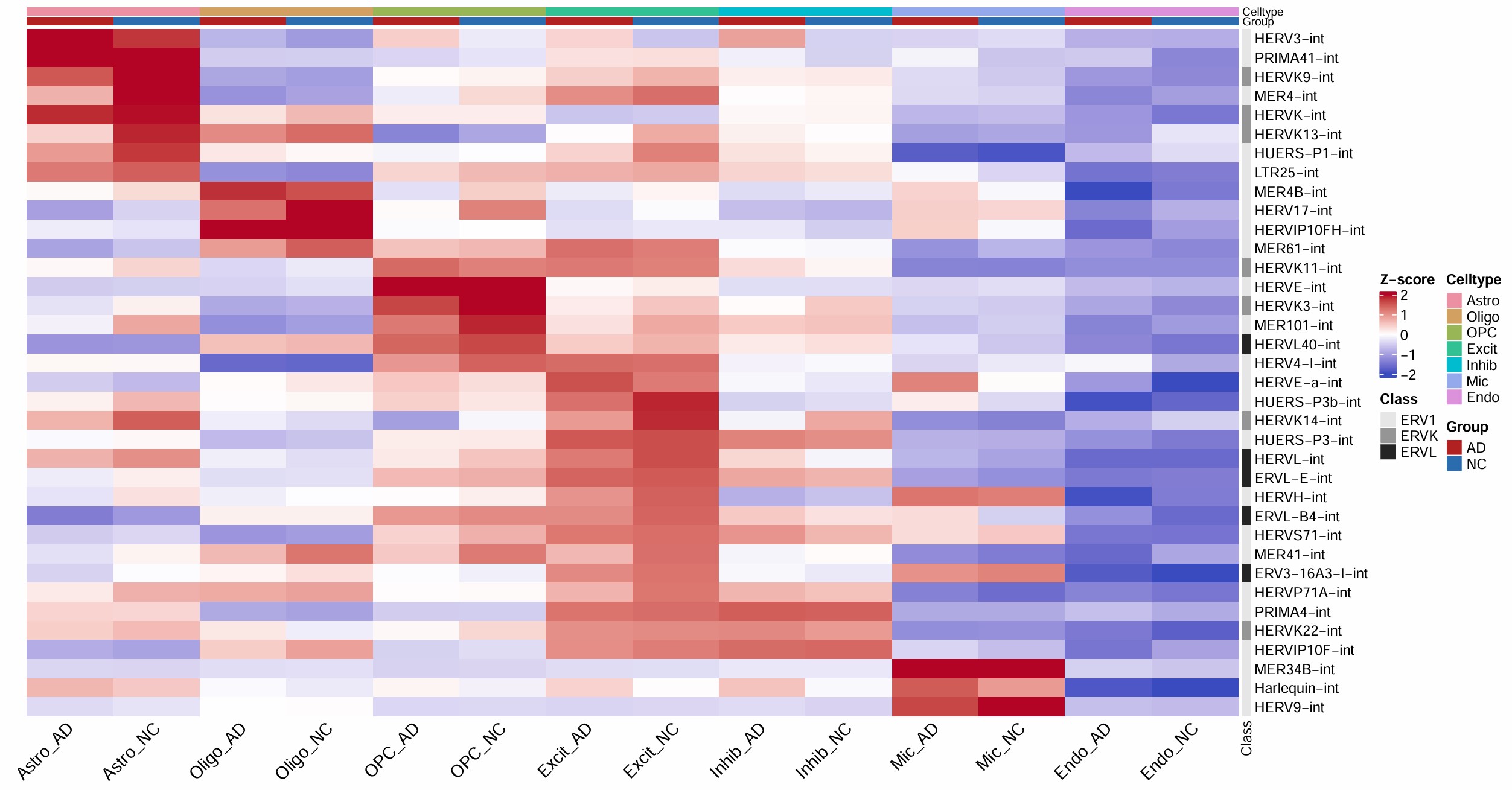
在我的研究中：只画热图，作为展示hERV整体分布的图。具体来说，把横轴的发育阶段换成Astro_NC/Astro_AD/Endo_NC/Endo_AD…，纵轴是是hERV家族（选一些高表达且在这些列之间变化较大的），右面加一个注释条标明超家族，先不做聚类，每个单元格的颜色表示该hERV家族在该细胞类型中的相对表达量，以此展示每个细胞类型中高表达的hERV有区别，经过测试，我选择了行标准化，即“同一个hERV家族在不同细胞类型中，哪里相对更高、哪里相对更低”（因为列标准化会出来很多hERV家族在所有细胞类型中表达都高，就没法体现出阶梯状的差异）

mat <- GetAssayData(seu, assay = "HERV_family", layer = "data")
celltype_order <- c("Astro", "Oligo", "OPC", "Excit", "Inhib", "Mic", "Endo")
group_order <- c("AD", "NC")
# 提取metadata，并构造列分组
meta <- seu@meta.data[, c("celltype", "group"), drop = FALSE]
mat <- mat[, rownames(meta), drop = FALSE]
meta$celltype <- factor(as.character(meta$celltype), levels = celltype_order)
meta$group <- factor(as.character(meta$group), levels = group_order)
mat <- mat[, rownames(meta), drop = FALSE]
meta$cellgroup <- paste(meta$celltype, meta$group, sep = "_")
col_order <- expand.grid(
  celltype = celltype_order,
  group = group_order,
  stringsAsFactors = FALSE
)
col_order$cellgroup <- paste(col_order$celltype, col_order$group, sep = "_")
col_order <- col_order[order(
  match(col_order$celltype, celltype_order),
  match(col_order$group, group_order)
), , drop = FALSE]
col_order <- col_order[col_order$cellgroup %in% meta$cellgroup, , drop = FALSE]
# 计算每个celltype×group的平均表达
avg_list <- lapply(col_order$cellgroup, function(x) {
  cells <- rownames(meta)[meta$cellgroup == x]
  Matrix::rowMeans(mat[, cells, drop = FALSE])
})
avg_mat <- do.call(cbind, avg_list)
colnames(avg_mat) <- col_order$cellgroup
rownames(avg_mat) <- rownames(mat)
# 选择“高表达且变化较大”的 hERV family
row_mean <- rowMeans(avg_mat)
row_sd <- apply(avg_mat, 1, sd)
min_mean <- 0.05  # “高表达”的阈值
top_n <- 40  # 画多少个family
keep <- row_mean >= min_mean
stat_df <- data.frame(
  family = rownames(avg_mat),
  mean_expr = row_mean,
  sd_expr = row_sd,
  stringsAsFactors = FALSE
)
stat_df <- stat_df[keep, ]
stat_df <- stat_df[order(-stat_df$sd_expr, -stat_df$mean_expr), ]  # 先按平均表达过滤，再按不同列之间的标准差排序
family_use <- head(stat_df$family, top_n)
plot_mat <- avg_mat[family_use, , drop = FALSE]
# 计算Z-score
plot_mat_z <- t(scale(t(as.matrix(plot_mat))))
plot_mat_z <- plot_mat_z[apply(plot_mat_z, 1, function(x) all(is.finite(x))), , drop = FALSE]
# 按“最高表达出现在哪一列”排序
peak_col <- max.col(plot_mat_z, ties.method = "first")
peak_val <- apply(plot_mat_z, 1, max)
ord <- order(peak_col, -peak_val)
plot_mat_z <- plot_mat_z[ord, , drop = FALSE]
# 加右侧超家族注释条
family_anno <- read.csv("/public/home/GENE_proc/wth/metadata/hERV/hERV_locus2family.csv")
family_anno$subfamily_raw <- gsub("_", "-", family_anno$subfamily_raw)
row_class <- family_anno$class[match(rownames(plot_mat_z), family_anno$subfamily_raw)]
row_class[is.na(row_class)] <- "Unknown"
class_cols <- c(
  "ERV1" = "#E6E6E6",
  "ERVK" = "#969696",
  "ERVL" = "#252525",
  "Unknown" = "#BDBDBD"
)
right_anno <- rowAnnotation(
  Class = row_class,
  col = list(Class = class_cols),
  show_annotation_name = TRUE,
  annotation_name_gp = gpar(fontsize = 10),
  simple_anno_size = unit(2, "mm")   # 右侧色条宽度
)
# 顶部注释
celltype_cols <- setNames(hcl.colors(length(celltype_order), "Set 2"), celltype_order)
group_cols <- c("NC" = "#2B6CB0", "AD" = "#B22222")
col_order$celltype <- factor(col_order$celltype, levels = celltype_order)  # 固定图例标签顺序
col_order$group <- factor(col_order$group, levels = group_order)
top_anno <- HeatmapAnnotation(
  Celltype = col_order$celltype,
  Group = col_order$group,
  col = list(
    Celltype = celltype_cols,
    Group = group_cols
  ),
  annotation_legend_param = list(
    Celltype = list(
      at = celltype_order
    ),
    Group = list(
      at = group_order
    )
  ),
  annotation_name_gp = gpar(fontsize = 8),
  simple_anno_size = unit(2, "mm")  # 顶部色条高度
  # , gap = unit(0.25, "mm")  # 两条注释之间留一点小空隙
)
# 画图
ht <- Heatmap(
  plot_mat_z,
  name = "Z-score",
  col = colorRamp2(c(-2, 0, 2), c("#3B4CC0", "white", "#B40426")),
  top_annotation = top_anno,
  right_annotation = right_anno,
  cluster_rows = FALSE,
  cluster_columns = FALSE,
  show_row_names = TRUE,
  show_column_names = TRUE,
  row_names_gp = gpar(fontsize = 10),
  column_names_gp = gpar(fontsize = 12),
  column_names_rot = 45,
  border = FALSE,
  # column_title = "Average expression of hERV families",
  # row_title = "hERV family",
  rect_gp = gpar(col = NA)  # 去掉单元格边框
)
pdf(file.path(res_dir, "hERV_family_heatmap.pdf"), width = 15, height = 8)
draw(ht, heatmap_legend_side = "right", annotation_legend_side = "right", padding = unit(c(5, 10, 5, 5), "mm"))
dev.off()

---

把z-score改成AD-NC的log2FC：即用hERV_family_celltype.csv画

de_df <- read_xlsx("C:\\Users\\17185\\Desktop\\hERV_AD_snRNA-seq_analyze\\res\\hERV_DE\\hERV_family_celltype.xlsx")
celltype_order <- c("Astro", "Oligo", "OPC", "Excit", "Inhib", "Mic", "Endo")
de_df <- de_df %>%
  filter(celltype %in% celltype_order) %>%
  select(celltype, subfamily, avg_log2FC)
logfc_df <- de_df %>%
  pivot_wider(
    names_from = celltype,
    values_from = avg_log2FC
  )
logfc_df <- logfc_df[, c("subfamily", celltype_order[celltype_order %in% colnames(logfc_df)])]
logfc_mat <- as.matrix(logfc_df[, -1])
rownames(logfc_mat) <- logfc_df$subfamily
logfc_mat[is.na(logfc_mat)] <- 0
row_sd <- apply(logfc_mat, 1, sd)
row_maxabs <- apply(abs(logfc_mat), 1, max)
stat_df <- data.frame(
  family = rownames(logfc_mat),
  sd_logFC = row_sd,
  max_abs_logFC = row_maxabs,
  stringsAsFactors = FALSE
)
stat_df <- stat_df[order(-stat_df$sd_logFC, -stat_df$max_abs_logFC), ]
top_n <- 40
family_use <- head(stat_df$family, top_n)
plot_mat <- logfc_mat[family_use, , drop = FALSE]
plot_mat_z <- t(scale(t(plot_mat)))
plot_mat_z[!is.finite(plot_mat_z)] <- 0
peak_col <- max.col(plot_mat_z, ties.method = "first")
peak_val <- apply(plot_mat_z, 1, max)
ord <- order(peak_col, -peak_val)
plot_mat <- plot_mat[ord, , drop = FALSE]
family_anno <- read.csv("C:\\Users\\17185\\Desktop\\hERV_AD_snRNA-seq_analyze\\metadata\\hERV\\hERV_locus2family.csv")
family_anno$subfamily_raw <- gsub("_", "-", family_anno$subfamily_raw)
row_class <- family_anno$class[match(rownames(plot_mat), family_anno$subfamily_raw)]
row_class[is.na(row_class)] <- "Unknown"
class_cols <- c(
  "ERV1" = "#E6E6E6",
  "ERVK" = "#969696",
  "ERVL" = "#252525",
  "Unknown" = "#BDBDBD"
)
right_anno <- rowAnnotation(
  Class = row_class,
  col = list(Class = class_cols),
  show_annotation_name = TRUE,
  annotation_name_gp = gpar(fontsize = 10),
  simple_anno_size = unit(2, "mm")
)
celltype_cols <- setNames(hcl.colors(length(celltype_order), "Set 2"), celltype_order)
top_anno <- HeatmapAnnotation(
  Celltype = factor(colnames(plot_mat), levels = celltype_order),
  col = list(Celltype = celltype_cols),
  annotation_legend_param = list(
    Celltype = list(at = celltype_order)
  ),
  annotation_name_gp = gpar(fontsize = 8),
  simple_anno_size = unit(2, "mm")
)
lim <- quantile(abs(plot_mat), 0.98, na.rm = TRUE)
lim <- max(lim, 0.2)
ht <- Heatmap(
  plot_mat,
  name = "log2FC",
  col = colorRamp2(c(-lim, 0, lim), c("#3B4CC0", "white", "#B40426")),
  top_annotation = top_anno,
  right_annotation = right_anno,
  cluster_rows = FALSE,
  cluster_columns = FALSE,
  show_row_names = TRUE,
  show_column_names = TRUE,
  row_names_gp = gpar(fontsize = 10),
  column_names_gp = gpar(fontsize = 12),
  column_names_rot = 45,
  border = FALSE,
  column_title = "logFC of hERV families All",
  # row_title = "hERV family",
  rect_gp = gpar(col = NA),
  na_col = "grey90",
)

组合图：

my_heatmap <- function(seu, de_res_path, herv_map_path = "/public/home/GENE_proc/wth/metadata/hERV/hERV_locus2family.csv"){
  dataset <- identity_seu(seu, "dataset")
  mat <- GetAssayData(seu, assay = "HERV_family", layer = "data")
  celltype_order <- c("Astro", "Oligo", "OPC", "Excit", "Inhib", "Mic", "Endo")
  group_order <- c("AD", "NC")
  meta <- seu@meta.data[, c("celltype", "group"), drop = FALSE]
  mat <- mat[, rownames(meta), drop = FALSE]
  meta$celltype <- factor(as.character(meta$celltype), levels = celltype_order)
  meta$group <- factor(as.character(meta$group), levels = group_order)
  mat <- mat[, rownames(meta), drop = FALSE]
  meta$cellgroup <- paste(meta$celltype, meta$group, sep = "_")
  col_order <- expand.grid(
    celltype = celltype_order,
    group = group_order,
    stringsAsFactors = FALSE
  )
  col_order$cellgroup <- paste(col_order$celltype, col_order$group, sep = "_")
  col_order <- col_order[order(
    match(col_order$celltype, celltype_order),
    match(col_order$group, group_order)
  ), , drop = FALSE]
  col_order <- col_order[col_order$cellgroup %in% meta$cellgroup, , drop = FALSE]
  avg_list <- lapply(col_order$cellgroup, function(x) {
    cells <- rownames(meta)[meta$cellgroup == x]
    Matrix::rowMeans(mat[, cells, drop = FALSE])
  })
  avg_mat <- do.call(cbind, avg_list)
  colnames(avg_mat) <- col_order$cellgroup
  rownames(avg_mat) <- rownames(mat)
  row_mean <- rowMeans(avg_mat)
  row_sd <- apply(avg_mat, 1, sd)
  min_mean <- 0.05
  top_n <- 40
  keep <- row_mean >= min_mean
  stat_df <- data.frame(
    family = rownames(avg_mat),
    mean_expr = row_mean,
    sd_expr = row_sd,
    stringsAsFactors = FALSE
  )
  stat_df <- stat_df[keep, ]
  stat_df <- stat_df[order(-stat_df$sd_expr, -stat_df$mean_expr), ]
  family_use <- head(stat_df$family, top_n)
  plot_mat <- avg_mat[family_use, , drop = FALSE]
  plot_mat_z <- t(scale(t(as.matrix(plot_mat))))
  plot_mat_z <- plot_mat_z[apply(plot_mat_z, 1, function(x) all(is.finite(x))), , drop = FALSE]
  peak_col <- max.col(plot_mat_z, ties.method = "first")
  peak_val <- apply(plot_mat_z, 1, max)
  ord <- order(peak_col, -peak_val)
  plot_mat_z <- plot_mat_z[ord, , drop = FALSE]
  family_anno <- read.csv(herv_map_path)
  family_anno$subfamily_raw <- gsub("_", "-", family_anno$subfamily_raw)
  row_class <- family_anno$class[match(rownames(plot_mat_z), family_anno$subfamily_raw)]
  row_class[is.na(row_class)] <- "Unknown"
  class_cols <- c(
    "ERV1" = "#E6E6E6",
    "ERVK" = "#969696",
    "ERVL" = "#252525",
    "Unknown" = "#BDBDBD"
  )
  right_anno <- rowAnnotation(
    Class = row_class,
    col = list(Class = class_cols),
    show_annotation_name = TRUE,
    annotation_name_gp = gpar(fontsize = 0),
    simple_anno_size = unit(2, "mm")
  )
  celltype_cols <- setNames(hcl.colors(length(celltype_order), "Set 2"), celltype_order)
  group_cols <- c("NC" = "#2B6CB0", "AD" = "#B22222")
  col_order$celltype <- factor(col_order$celltype, levels = celltype_order)
  col_order$group <- factor(col_order$group, levels = group_order)
  top_anno <- HeatmapAnnotation(
    Celltype = col_order$celltype,
    Group = col_order$group,
    col = list(
      Celltype = celltype_cols,
      Group = group_cols
    ),
    annotation_legend_param = list(
      Celltype = list(
        at = celltype_order
      ),
      Group = list(
        at = group_order
      )
    ),
    annotation_name_gp = gpar(fontsize = 0),
    simple_anno_size = unit(2, "mm")
  )
  up <- Heatmap(
    plot_mat_z,
    name = "Z-score",
    col = colorRamp2(c(-2, 0, 2), c("#3B4CC0", "white", "#B40426")),
    top_annotation = top_anno,
    right_annotation = right_anno,
    cluster_rows = FALSE,
    cluster_columns = FALSE,
    show_row_names = TRUE,
    show_column_names = FALSE,
    row_names_gp = gpar(fontsize = 10),
    column_names_rot = 45,
    border = FALSE,
    column_title = paste0("Average expression of hERV families - ", dataset),
    column_title_gp = gpar(fontsize = 16),
    rect_gp = gpar(col = NA)
  )
  de_df <- read.csv(de_res_path)
  de_df <- de_df %>%
    filter(celltype %in% celltype_order) %>%
    select(celltype, subfamily, avg_log2FC)
  logfc_df <- de_df %>%
    pivot_wider(
      names_from = celltype,
      values_from = avg_log2FC
    )
  logfc_df <- logfc_df[, c("subfamily", celltype_order[celltype_order %in% colnames(logfc_df)])]
  logfc_mat <- as.matrix(logfc_df[, -1])
  rownames(logfc_mat) <- logfc_df$subfamily
  row_sd <- apply(logfc_mat, 1, sd)
  row_maxabs <- apply(abs(logfc_mat), 1, max)
  stat_df <- data.frame(
    family = rownames(logfc_mat),
    sd_logFC = row_sd,
    max_abs_logFC = row_maxabs,
    stringsAsFactors = FALSE
  )
  stat_df <- stat_df[order(-stat_df$sd_logFC, -stat_df$max_abs_logFC), ]
  top_n <- 40
  family_use <- head(stat_df$family, top_n)
  plot_mat <- logfc_mat[family_use, , drop = FALSE]
  plot_mat_z <- t(scale(t(plot_mat)))
  plot_mat_z[!is.finite(plot_mat_z)] <- 0
  peak_col <- max.col(plot_mat_z, ties.method = "first")
  peak_val <- apply(plot_mat_z, 1, max)
  ord <- order(peak_col, -peak_val)
  plot_mat <- plot_mat[ord, , drop = FALSE]
  row_class <- family_anno$class[match(rownames(plot_mat), family_anno$subfamily_raw)]
  row_class[is.na(row_class)] <- "Unknown"
  right_anno <- rowAnnotation(
    Class = row_class,
    col = list(Class = class_cols),
    show_annotation_name = TRUE,
    annotation_name_gp = gpar(fontsize = 0),
    simple_anno_size = unit(2, "mm")
  )
  celltype_cols <- setNames(hcl.colors(length(celltype_order), "Set 2"), celltype_order)
  top_anno <- HeatmapAnnotation(
    Celltype = factor(colnames(plot_mat), levels = celltype_order),
    col = list(Celltype = celltype_cols),
    annotation_legend_param = list(
      Celltype = list(at = celltype_order)
    ),
    annotation_name_gp = gpar(fontsize = 0),
    simple_anno_size = unit(2, "mm")
  )
  lim <- quantile(abs(plot_mat), 0.98, na.rm = TRUE)
  lim <- max(lim, 0.2)
  down <- Heatmap(
    plot_mat,
    name = "log2FC",
    col = colorRamp2(c(-lim, 0, lim), c("#3B4CC0", "white", "#B40426")),
    top_annotation = top_anno,
    right_annotation = right_anno,
    cluster_rows = FALSE,
    cluster_columns = FALSE,
    show_column_names = FALSE,
    show_row_names = TRUE,
    row_names_gp = gpar(fontsize = 10),
    border = FALSE,
    column_title = paste0("logFC of hERV families - ", dataset),
    column_title_gp = gpar(fontsize = 16),
    rect_gp = gpar(col = NA),
    na_col = "grey90",
  )
  up <- as.ggplot(up)
  down <- as.ggplot(down)
  pdf(file.path(res_dir, paste0("hERV_family_heatmap_", dataset, ".pdf")), width = 10, height = 12)
  print(up / down)
  dev.off()
}

其它问题

dotplot表达量负数

Average Expression：经过标准化后的平均表达量。DotPlot默认会对每个基因在不同细胞群之间的平均表达做缩放，缩放之后，数值表示的是这个基因在某个群里的表达，相对于该基因在所有群中的整体水平是高还是低：

• 大于0：这个群里该基因表达高于该基因的整体平均水平
• 小于0：这个群里该基因表达低于该基因的整体平均水平
• 0附近：接近平均水平

如果在DotPlot设置参数scale = FALSE，就是原始平均表达量

测序方法对hERV计数的影响

使用的数据的建库方法是10x Chromium Single Cell 3′ v3——“用poly(dT)引物捕获带poly(A)尾的转录本”，可能会低估或者漏掉不带polyA的ncRNA（非编码RNA），同时TE里面有相当一部分是non-polyA的，所以在hERV计数上大概率会偏低。不过我这个分析主要是AD-NC/不同细胞类型之间的组间比较，或者是共表达这种定性的找趋势，所以在这类不需要精确计数的分析上应该影响不大。当然也不可能说完全没有影响：

• 之前别人的bulk RNA-seq分析用的是total RNA的测序方法（而不是我这种polyA+的测序方法），这可能是结论有差异的原因之一
• 我这里能被polyA+的测序方法测出来的hERV读段，可能是hERV中有一定特殊性的片段，比如是剪接到了正常gene中的、或是借用了周围的polyA

hERV被基因内化为外显子或是启动子/增强子对测序的影响：

• 内化为外显子：更偏向polyA+，因为这时它本质上已经成了宿主基因转录本的一部分，后续剪接、加polyA、输出等过程大多按宿主mRNA或某些lncRNA的规则来走
• 内化为替代启动子：也常常更偏向polyA+，因为很多情况下是 LTR 驱动了一个宿主基因的替代转录本，这个转录本后面接宿主外显子，最后通常会形成比较稳定的加polyA尾的RNA
• 内化为增强子：更偏向non-polyA，因为增强子大多数不产生稳定RNA

古老型hERV更容易被基因内化为外显子或是启动子/增强子？

• 总体上，较老的TE/ERV更容易在进化中被宿主共选为调控元件。比如hERVK(HML-2)属于hERV中较年轻、最接近仍保留病毒样转录潜力的家族之一，而hERVL/ERVL就属于更古老的谱系，但在同一家族内部，也会有一些特殊的位点（比如hERVH就有一些年轻的高转录位点）
• hERV的年龄更可能改变“它以什么形式被转录出来”，而不是直接规定它一定是polyA还是non-polyA
  • 古老型如果更多作为外显子/启动子（被内化进宿主基因转录本），polyA+比例会上升
  • 古老型如果更多作为增强子产生调控RNA，non-polyA比例会上升
  • 年轻型如果更多保持自主病毒样转录，polyA+也可能很高
• polyA测序更容易检测到
  • 嵌在宿主polyA转录本里的hERV片段
  • 本身能形成polyA尾的hERV转录本
• 从热图上看，也是既有ERVL/HERVL，也有hERVK这类，似乎并没有说高表达的更偏向年轻/古老

Human hippocampal neurogenesis

Human hippocampal neurogenesis in adulthood, ageing and Alzheimer’s disease

主要结论：成人海马神经发生是存在的；AD不只是“新生神经元少了”，更像是从前体细胞开始，整条神经发生轴线的表观调控网络逐步失稳；而认知保持得特别好的人，保留了一套与这种失稳相反的“韧性网络”

• 人类成年海马确实存在一条可识别的神经发生轨迹：用snRNA-seq和snATAC-seq联合分析，识别出了NSCs（神经干细胞）、neuroblasts（神经母细胞）、immature neurons（未成熟神经元），并且通过RNA velocity和调控网络分析支持它们构成一条从干/祖细胞到未成熟神经元的连续轨迹
• 随着衰老和AD进展，最稳定、最明显的变化不是RNA，而是染色质开放性：与DEGs相比，DARs（差异染色质开放区域）的变化更多、更强，也更能区分正常衰老、临床前阶段和AD。尤其在PCI（可理解为向AD过渡的临床前病理状态）里，一些和突触可塑性、神经传递、神经元结构维护有关的开放染色质区域已经开始下调，而这些变化在AD中更严重
• 最早的异常更可能起始于NSC，后面在neuroblast和immature neuron里放大
• SuperAgers（在情景记忆测试中表现出色的老年人）有更独特的neurogenesis profile，尤其是在immature neurons/neuroblasts上更明显，而且这种“resilience signature”主要也是体现在开放染色质和调控网络上，这种韧性与海马内astrocytes、CA1 neurons、谷氨酸能突触通路之间的相互作用有联系，“认知功能未明显衰退”和“认知衰退”分岔点可能就在这些细胞间调控网络上

TE和免疫系统

Transposable elements as instructors of the immune system

主要结论：TE在多个层面作为免疫系统行为的调控元件

• TE被转录后产生RNA、cDNA、蛋白或肽段，这些产物能被先天免疫识别，或者被MHC呈递给T细胞
• TE还能作为顺式调控元件，重塑某些免疫细胞的基因表达程序，或充当某些免疫细胞状态转换和组织适应程序中的增强子：免疫系统可能反复利用TE作为调控方式
  • TE转录出来的RNA或RNA-DNA产物可以激活RIG-I、MDA5、cGAS–STING等先天免疫通路，从而诱导I型干扰素反应
  • 在T细胞里，某些含LINE-1的转录本和T细胞的活化、分化、耗竭状态有关
  • 在胸腺里，TE来源的转录本和肽段甚至可能参与中枢耐受，防止免疫系统攻击自身正常细胞
  • 某些ERV类TE影响辅助性T细胞分化
  • 在不同组织免疫细胞的scATAC-seq里找到了一批与组织适应有关的TE家族/亚家族，发现这些TE所在开放染色质里富集了BATF、JUNB等关键转录因子结合位点
• 未来可能用于癌症免疫治疗，也可能用于炎症和自身免疫病的干预

TE增强子调控网络如何计算：

• 先找候选增强子：用ATAC-seq或scATAC-seq找开放染色质区域
• 把开放峰和TE注释重叠：把ATAC峰和RepeatMasker之类的TE注释表相交，筛出“落在TE上的开放峰”，这些就是候选的TE-derived enhancers。然后再统计哪些TE家族/亚家族在某个细胞状态中显著富集
• motif enrichment推断谁在用这些TE：如果某些开放的TE峰里富集BATF、JUNB、TH1相关TF（转录因子）的motif（序列中的特定模式），就提示这些TF可能通过这些TE位点来驱动该细胞程序
• 把峰连到基因：做peak-gene correlation、co-accessibility，或者用同一细胞的RNA+ATAC多组学数据去关联“这个开放峰变化”和“哪个基因表达变化同步”
• 把这些关系拼成网络，并做实验验证

JETs（外显子和TE序列拼接形成的非经典转录本）在肿瘤里已经显示出很有意思的抗原潜力：一些肿瘤特异的JETs可以被翻译成蛋白，并作为肽段经MHC-I呈递，还能诱导T细胞反应。虽然他还没有被证实为神经系统疾病标志物，不过潜力很大